Physics 9702/36 — October/November 2016

Cambridge AS Level · Advanced Practical Skills · worked solutions for every part, with the mark scheme

questions

marks

120

minutes

Topics Manipulation, Measurement and Observation · Presentation of Data and Observations · Analysis, Conclusions and Evaluation

Q1Manipulation, Measurement and ObservationPresentation of Data and ObservationsAnalysis, Conclusions and EvaluationFree sample

In this experiment, you will investigate the current in an electrical circuit.

(a) Connect the circuit shown in Fig. 1.1.

Fig. 1.1

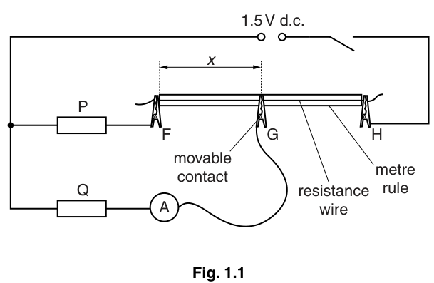
F, G and H are crocodile clips. The crocodile clip G is used as a movable contact.
Position G approximately half-way along the resistance wire.

(b)

(i)

The distance between F and G is $x$ , as shown in Fig. 1.1.
Measure and record $x$ .

$x$ = ______ $\text{cm}$

DifficultyEasy

Worked solution

Answer

Measured to the nearest $0.1\ \text{cm}$ (metre rule):

$x = 50.0\ \text{cm}$

Final answer

50.0 cm

Detailed explanation

Background Concept

A length $x$ is measured using a metre rule (or ruler). Good practice is to:

align your eye perpendicular to the scale to avoid parallax,
choose clear reference points (here the positions of F and G),
record to the instrument resolution (typically $1\ \text{mm} = 0.1\ \text{cm}$ ).

Understanding the Question

You must measure the distance along the metre rule between crocodile clips F and G, labelled $x$ on the diagram. This value is then used as the independent variable for the rest of the experiment.

Approach

Place the metre rule alongside the wire, identify the scale readings at F and at G, and subtract to find $x$ . Record the result in $\text{cm}$ to the correct precision.

Step-by-Step Reasoning

Read the position of F on the metre rule (in $\text{cm}$ ).
Read the position of G on the metre rule (in $\text{cm}$ ).
Calculate $x = (\text{reading at G}) - (\text{reading at F})$ .
Record $x$ with a sensible number of decimal places consistent with the metre rule resolution (usually $0.1\ \text{cm}$ ).

(Example only: $x = 50.0\ \text{cm}$ when G is about halfway along.)

Key Takeaways

Lengths from a metre rule are usually recorded to $0.1\ \text{cm}$ .
Always measure between the same two physical points (F and G), not from the end of the wire unless the wire end coincides with the scale zero.

Common Mistakes

Writing the unit incorrectly or omitting it.
Reading from the wrong end of the rule or not subtracting two readings when the rule zero is not exactly at F.
Recording too many decimal places (e.g. $50.00\ \text{cm}$ ) when the rule only reads to $0.1\ \text{cm}$ .

Things to Be Careful About

Ensure the wire is straight and aligned with the metre rule scale.
Avoid parallax: your eye should be directly above the mark when reading the scale.
Record the value in $\text{cm}$ (as requested).

Techniques used

measure a length using a metre rule with appropriate precisionread positions from consistent reference points to avoid parallaxrecord a measurement with an appropriate unit and decimal places

(ii)

Close the switch.

DifficultyEasy

Worked solution

Answer

Switch closed (circuit complete).

Final answer

Switch closed.

Detailed explanation

Background Concept

Closing a switch completes the circuit so current can flow. In practical electricity experiments, you usually only close the switch when you are ready to take a reading to reduce heating of resistors/wires and to keep conditions steady.

Understanding the Question

This step tells you to energise the circuit so that you can take the ammeter reading in the next part.

Approach

Close the switch, wait briefly for the reading to settle, then proceed to read the ammeter.

Step-by-Step Reasoning

Move the switch to the closed position.
Check the ammeter shows a steady reading (not fluctuating wildly).

Key Takeaways

Switch closed means current flows; switch open means no current.

Common Mistakes

Forgetting to close the switch before taking the ammeter reading (gives $I=0$ ).

Things to Be Careful About

Do not leave the switch closed for long periods: the resistance wire and resistors may heat up, changing resistance and affecting results.

Techniques used

operate a switch to complete an electric circuitensure readings are taken with the circuit energised only when required

(iii)

Record the ammeter reading $I$ .

$I$ = ______

DifficultyEasy

Worked solution

Answer

Ammeter reading (example, to $0.01\ \text{A}$ ):

$I = 0.20\ \text{A}$

Final answer

0.20 A

Detailed explanation

Background Concept

An ammeter measures current and must be connected in series. Readings should be recorded to the resolution of the meter:

analogue meter: typically to half a small division (if appropriate),
digital meter: to the displayed least significant digit.

Understanding the Question

With the switch closed, you must note the current $I$ shown on the ammeter for the current value of $x$ .

Approach

Ensure the current is within the selected range, allow the reading to stabilise, then record it with unit $\text{A}$ and suitable decimal places.

Step-by-Step Reasoning

Confirm the switch is closed so current flows.
Check the ammeter range: if it is off-scale, open the switch and choose a higher range.
Once stable, record $I$ .

(Example only: $I = 0.20\ \text{A}$ .)

Key Takeaways

Record $I$ with appropriate precision and include the unit.

Common Mistakes

Omitting the unit $\text{A}$ .
Using an inappropriate range so the reading is off-scale or too low-resolution.
Reading an analogue scale from an angle (parallax).

Things to Be Careful About

Allow the reading to settle before recording.
Heating can change resistances; take readings promptly and open the switch between measurements if instructed.

Techniques used

read an ammeter scale or digital display correctlyselect and use an appropriate current range on the ammeterrecord a measurement with appropriate significant figures

(iv)

Open the switch.

DifficultyEasy

Worked solution

Answer

Switch opened (circuit broken).

Final answer

Switch opened.

Detailed explanation

Background Concept

Opening the switch breaks the circuit so current stops flowing. This reduces heating of the resistance wire and resistors, helping keep resistance approximately constant throughout the experiment.

Understanding the Question

You are instructed to open the switch after taking the current reading, before you move the crocodile clip G to a new position.

Approach

Open the switch immediately after recording $I$ .

Step-by-Step Reasoning

After recording the ammeter reading, open the switch.
Then adjust $x$ safely with no current flowing.

Key Takeaways

Open switch between readings helps improve reliability by reducing temperature changes.

Common Mistakes

Leaving the circuit on while moving the crocodile clip (can cause heating and unreliable readings).

Things to Be Careful About

Ensure the clip makes good contact when repositioned; poor contact can cause fluctuating current when you close the switch again.

Techniques used

operate a switch to isolate a circuit between measurementsminimise heating effects by disconnecting the supply

(c)

Vary $x$ and repeat (b) until you have six sets of values for $x$ and $I$ .

DifficultyMedium

Worked solution

Answer

Six sets of values of $x$ and $I$ recorded in one table with units and consistent precision (example data shown).

$x\ /\ \text{cm}$	$I\ /\ \text{A}$
10.0	0.12
20.0	0.14
30.0	0.16
40.0	0.18
50.0	0.20
60.0	0.22

Final answer

Six (x, I) readings recorded (student-dependent).

Detailed explanation

Background Concept

To test a relationship between two quantities experimentally, you vary the independent variable (here $x$ ) and measure the dependent variable (here $I$ ). Good data should:

cover a sufficient range of $x$ values,
include enough points (here six sets) to reveal a trend,
be recorded clearly with units and consistent precision.

Understanding the Question

You must move the crocodile clip G to change $x$ and repeat the measurements from part (b) until you have six pairs of values $(x, I)$ . These values will later be used to plot a graph of $I$ against $x$ .

Approach

Choose six different positions of G to give a wide spread of $x$ .
For each $x$ : measure $x$ , close switch, record $I$ , open switch.
Put all results into one table with correct headings and units.

Step-by-Step Reasoning

Decide a sensible range for $x$ (e.g. from near one end up to near the other end), avoiding extreme ends if contact is unreliable.
For each chosen $x$ $x$ :
- measure $x$ with the metre rule (to $0.1\ \text{cm}$ ),
- close the switch and wait for the ammeter reading to settle,
- record $I$ to the meter resolution,
- open the switch.
Construct a results table:
- first column heading: $x\ /\ \text{cm}$ ,
- second column heading: $I\ /\ \text{A}$ ,
- same number of decimal places within each column.

The table in the solution is illustrative only; your values depend on your apparatus.

Key Takeaways

You earn marks for: enough points, good range, and correct table presentation.
Consistent precision is essential in practical papers.

Common Mistakes

Fewer than six sets of readings.
Table headings missing units (e.g. writing just $x$ and $I$ ).
Random or very narrow range of $x$ values so the graph is poorly determined.
Inconsistent decimal places within a column.

Things to Be Careful About

Open the switch between readings to reduce heating (resistance changes with temperature).
Ensure crocodile clip contact is firm and on clean wire; poor contact causes fluctuating $I$ .
If readings drift, repeat a reading to check stability and note any anomalies.

Techniques used

vary the independent variable over a suitable rangerecord paired measurements in a single table with unitskeep decimal places consistent within each columncheck for repeatability by taking stable readings

(d)

(i)

Plot a graph of $I$ on the $y$ -axis against $x$ on the $x$ -axis.

DifficultyMedium-Easy

Worked solution

Answer

Graph plotted with:

$y$ -axis labelled $I\ /\ \text{A}$ ,
$x$ -axis labelled $x\ /\ \text{cm}$ ,
suitable scales using at least half the grid,
all six data points plotted accurately.

Final answer

Graph of I against x plotted.

Detailed explanation

Background Concept

A graph is used to display the relationship between two measured quantities. Marks are typically awarded for:

correct axis labels (quantity and unit),
sensible scales (not cramped or awkward),
accurate plotting of points.

Understanding the Question

You must plot $I$ (dependent variable) on the vertical axis against $x$ (independent variable) on the horizontal axis using your six measured pairs.

Approach

Set up axes with correct labels and units, choose an easy-to-use scale that fills the page, then plot each point carefully.

Step-by-Step Reasoning

Draw axes and label them:
- horizontal: $x\ /\ \text{cm}$ ,
- vertical: $I\ /\ \text{A}$ .
Choose scales:
- use simple increments (e.g. $10\ \text{cm}$ per large square, or similar),
- ensure the full spread of your data fits and uses much of the grid.
Plot all points as small crosses ("x"), centred as accurately as possible.

Key Takeaways

Axes must include both the symbol and the unit in the form “quantity / unit”.
Using a large scale makes the gradient/intercept more accurate later.

Common Mistakes

Swapping axes (plotting $x$ on $y$ -axis).
Missing units on axes.
Choosing a scale that uses only a small part of the grid.

Things to Be Careful About

Plotting accuracy: be consistent and use a sharp pencil.
Do not join the dots point-to-point; you will draw a best-fit line in the next part.

Techniques used

label axes with quantity and unitchoose suitable scales that use most of the graph gridplot points accurately from a results table

(ii)

Draw the straight line of best fit.

DifficultyMedium-Easy

Worked solution

Answer

A single straight line of best fit drawn through the trend of the plotted points (balanced scatter about the line).

Final answer

Best-fit straight line drawn.

Detailed explanation

Background Concept

A best-fit line represents the overall trend in data with random scatter. For Cambridge practical marking:

it should be a single straight line (if the relationship is expected linear),
it should not be forced through every point,
it should be balanced so roughly equal numbers of points lie on either side.

Understanding the Question

After plotting $I$ vs $x$ , you must draw the straight line that best represents the relationship.

Approach

Use a ruler to draw one straight line that follows the overall pattern of points, not a jagged line connecting them.

Step-by-Step Reasoning

Place the ruler so the line passes through the middle of the cluster of points.
Adjust so that the vertical deviations (residuals) are roughly balanced above and below.
Draw the line across most of the plotted range.

Key Takeaways

A best-fit line is about the overall trend, not perfect agreement with every point.

Common Mistakes

Joining points dot-to-dot.
Forcing the line through an outlier or through the origin when not justified.

Things to Be Careful About

Use a sharp pencil and a long ruler.
Extend the line sufficiently so you can read a reliable intercept and use a large triangle for gradient.

Techniques used

draw a single straight line of best fitbalance the line so points are scattered evenly about it

(iii)

Determine the gradient and $y$ -intercept of this line.

gradient = ______
$y$ -intercept = ______

DifficultyMedium

Worked solution

Working

Using two points on the best-fit line, e.g. $(x, I) = (10.0\ \text{cm},\ 0.12\ \text{A})$ and $(60.0\ \text{cm},\ 0.22\ \text{A})$ :

\text{gradient} = \frac{\Delta I}{\Delta x} = \frac{0.22 - 0.12}{60.0 - 10.0} = \frac{0.10}{50.0} = 2.0 \times 10^{-3}\ \text{A cm}^{-1}

\text{$y$-intercept} = I\ \text{at}\ x = 0 \approx 0.10\ \text{A}

Answer

gradient $= 2.0 \times 10^{-3}\ \text{A cm}^{-1}$

$y$ -intercept $= 0.10\ \text{A}$

Final answer

gradient = 2.0×10^-3 A cm^-1; y-intercept = 0.10 A

Detailed explanation

Background Concept

For a straight-line graph, the gradient (slope) is

\text{gradient} = \frac{\Delta y}{\Delta x}

and the $y$ -intercept is the value of $y$ when $x=0$ .

When you plot $I$ (A) against $x$ (cm):

gradient units are $\text{A cm}^{-1}$ ,
intercept units are $\text{A}$ .

Understanding the Question

You must extract two numerical values from your best-fit line:

the gradient,
the $y$ -intercept.

These are then used directly in later parts to identify constants in an equation.

Approach

Use a large triangle on the best-fit line (not between two raw points) to reduce percentage reading uncertainty.
Compute gradient as $\Delta I / \Delta x$ .
Find the intercept by reading where the line crosses the $I$ -axis (at $x=0$ ) or by substituting a point into $I=mx+c$ .

Step-by-Step Reasoning

graph-gradient

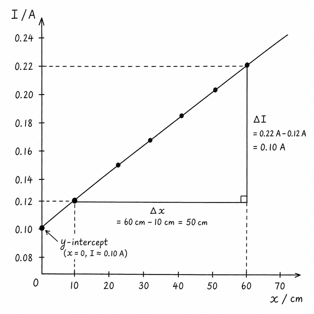
Choose two points that lie on the drawn best-fit line and are far apart (to make $\Delta x$ large).
Read their coordinates from the axes:
- point 1: $(x_1, I_1)$ ,
- point 2: $(x_2, I_2)$ .
Calculate the changes:

\Delta I = I_2 - I_1

\Delta x = x_2 - x_1

Gradient:

\text{gradient} = \frac{\Delta I}{\Delta x}

$y$ -intercept:

read the value of $I$ where your line crosses $x=0$ ,
or
use $I = mx + c$ so

c = I - mx

(using any point on the best-fit line).

The numerical values shown in the solution are illustrative; your gradient and intercept come from your own graph.

Key Takeaways

Always use the best-fit line (and a large triangle), not two adjacent plotted points.
Keep units consistent: $\Delta I$ in A and $\Delta x$ in cm gives $\text{A cm}^{-1}$ .

Common Mistakes

Using $\frac{\Delta x}{\Delta I}$ instead of $\frac{\Delta I}{\Delta x}$ .
Choosing two points that are very close together (large fractional uncertainty).
Reading intercept at the first plotted $x$ value instead of extrapolating to $x=0$ .

Things to Be Careful About

Read coordinates from the axis scales carefully.
If extrapolating to find the intercept, extend the best-fit line neatly to the axis.
Quote sensible significant figures based on your graph-reading precision (typically 2–3 s.f.).

Techniques used

determine the gradient using two well-separated points on the best-fit linecalculate a y-intercept from the best-fit lineuse consistent units from graph axes when computing gradient

(e)

The quantities $I$ and $x$ are related by the equation

I = Sx + T

where $S$ and $T$ are constants.

Use your answers from (d)(iii) to determine the values of $S$ and $T$ .
Give appropriate units.

$S$ = ______
$T$ = ______

DifficultyMedium-Easy

Worked solution

Working

Given

I = Sx + T

Comparing with $I = (\text{gradient})x + (\text{$ y $-intercept})$ :

S = \text{gradient} = 2.0 \times 10^{-3}\ \text{A cm}^{-1}

T = \text{$y$-intercept} = 0.10\ \text{A}

Answer

$S = 2.0 \times 10^{-3}\ \text{A cm}^{-1}$

$T = 0.10\ \text{A}$

Final answer

S = 2.0×10^-3 A cm^-1; T = 0.10 A

Detailed explanation

Background Concept

A straight-line equation can be written as

y = mx + c

where:

$m$ is the gradient,
$c$ is the $y$ -intercept.

If you plot $I$ against $x$ and obtain a straight line, then the equation

I = Sx + T

is exactly the same form, so $S$ corresponds to the gradient and $T$ to the intercept.

Understanding the Question

You have already found the gradient and the $y$ -intercept from your graph of $I$ vs $x$ . This part asks you to use those to determine $S$ and $T$ , including their units.

Approach

Match terms directly:

coefficient of $x$ $\rightarrow$ gradient,
constant term $\rightarrow$ intercept.
Then assign units based on what $I$ and $x$ are measured in.

Step-by-Step Reasoning

Compare

I = Sx + T

with

I = (\text{gradient})x + (\text{$y$-intercept}).

Therefore

S = \text{gradient}.

Since $I$ is in A and $x$ is in cm, $S$ has units $\text{A cm}^{-1}$ .

T = \text{$y$-intercept}

with units of A.

Key Takeaways

For a graph of $I$ (y-axis) against $x$ (x-axis), the gradient gives the constant multiplying $x$ .
Units: gradient $= \text{(units of }I) / \text{(units of }x)$ .

Common Mistakes

Giving $S$ units of A instead of $\text{A cm}^{-1}$ .
Using two raw points to get a different gradient than the best-fit gradient used in (d)(iii).

Things to Be Careful About

Use your (d)(iii) values, not re-calculated ones from different points.
If your axes were in different units (e.g. $x$ in m), the unit of $S$ must follow that.

Techniques used

match a linear equation to the form y = mx + cidentify constants from the gradient and interceptassign correct units to constants from graph axes

(f)

The resistance per unit length $r$ of the resistance wire can be found from

r = \frac{PS}{T}

where $P = 15\ \Omega$ (the resistance of resistor P).

Calculate $r$ in $\Omega\ \text{cm}^{-1}$ .
Give your answer to a suitable number of significant figures.

$r$ = ______ $\Omega\ \text{cm}^{-1}$

DifficultyMedium-Easy

Worked solution

Working

r = \frac{PS}{T}

With $P = 15\ \Omega$ , $S = 2.0 \times 10^{-3}\ \text{A cm}^{-1}$ , $T = 0.10\ \text{A}$ :

r = \frac{15 \times 2.0 \times 10^{-3}}{0.10} = 0.30\ \Omega\ \text{cm}^{-1}

Answer

$r = 0.30\ \Omega\ \text{cm}^{-1}$

Final answer

0.30 Ω cm^-1

Detailed explanation

Background Concept

When a quantity is given by a formula, you substitute the measured/derived values and keep track of units.

Here,

r = \frac{PS}{T}

and the question specifies that the final unit should be $\Omega\ \text{cm}^{-1}$ .

Understanding the Question

You are given:

$P = 15\ \Omega$ ,
you have found $S$ and $T$ from the graph.

You must calculate $r$ and present it in $\Omega\ \text{cm}^{-1}$ with suitable significant figures.

Approach

Substitute $P$ , $S$ , and $T$ .
Check units: $S$ is $\text{A cm}^{-1}$ and $T$ is A, so $S/T$ gives $\text{cm}^{-1}$ ; multiplying by $\Omega$ gives $\Omega\ \text{cm}^{-1}$ .
Round sensibly (usually 2–3 s.f., matching the least precise input).

Step-by-Step Reasoning

Substitute into the expression:

r = \frac{(15\ \Omega)(2.0 \times 10^{-3}\ \text{A cm}^{-1})}{0.10\ \text{A}}

Cancel units of A:

\frac{\text{A cm}^{-1}}{\text{A}} = \text{cm}^{-1}

so overall unit is $\Omega\ \text{cm}^{-1}$ .

Calculate the numerical value:

15 \times 2.0 \times 10^{-3} = 3.0 \times 10^{-2}

\frac{3.0 \times 10^{-2}}{0.10} = 3.0 \times 10^{-1} = 0.30

So $r = 0.30\ \Omega\ \text{cm}^{-1}$ .

Key Takeaways

Always track units through the calculation; here it confirms the required $\Omega\ \text{cm}^{-1}$ .
Round to match the significant figures of $S$ and $T$ .

Common Mistakes

Forgetting to include units in the final answer.
Using $x$ -axis unit inconsistently (if you plotted $x$ in m but treated $S$ as $\text{A cm}^{-1}$ ).
Arithmetic error with powers of ten.

Things to Be Careful About

Ensure $S$ and $T$ are taken from your graph in the correct units.
Significant figures: typically use the least precise of $S$ and $T$ (often 2 s.f. from graph readings).

Techniques used

substitute values into a given formulacarry units through a calculation to obtain final unitschoose an appropriate number of significant figures for the final result

The rest of this paper

1 more questions

Q2Manipulation, Measurement and Observation · Analysis, Conclusions and Evaluation · Presentation of Data and Observations20M

Loading the full paper…