Physics 9702/34 — October/November 2016

Cambridge AS Level · Advanced Practical Skills · worked solutions for every part, with the mark scheme

questions

marks

120

minutes

Topics Manipulation, Measurement and Observation · Presentation of Data and Observations · Analysis, Conclusions and Evaluation

Q1Manipulation, Measurement and ObservationPresentation of Data and ObservationsAnalysis, Conclusions and EvaluationFree sample

In this experiment, you will investigate the oscillations of a wooden strip.

(a) Set up the apparatus as shown in Fig. 1.1, with the distance $x$ approximately equal to 25 cm.

Fig. 1.1

(b)

(i)

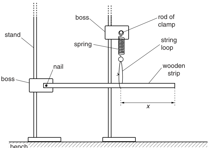
Ensure that the spring is vertical and the wooden strip is parallel to the bench.

DifficultyEasy

Worked solution

Answer

Adjust the clamps/stands so that the spring hangs vertically and the wooden strip is parallel to the bench (level).

Final answer

Spring vertical; strip parallel to bench.

Detailed explanation

Background Concept

For oscillation experiments, the motion should occur in the intended plane/line only. If the spring is not vertical or the strip is not level, additional components of force/torque appear, which can change the period and increase scatter in the data.

Understanding the Question

You are told to ensure two alignment conditions before measuring anything:

the spring must hang straight down (its axis vertical),
the wooden strip must be parallel to the bench (not tilted).
These reduce systematic errors and help the strip oscillate cleanly.

Approach

Make small adjustments to the positions of the stands/clamps until the spring is vertical and the strip is level. Then re-check after attaching the string loop, since the load may pull the spring sideways.

Step-by-Step Reasoning

With the spring attached, look from the side and front; adjust the stand positions so the spring does not lean.
Ensure the string loop pulls along the strip without twisting it.
Check the strip height at two points above the bench (near the support and near the free end). Adjust the boss/clamp height until these are the same, so the strip is parallel to the bench.
Re-check: a small misalignment can produce sideways oscillations and inconsistent timing.

Key Takeaways

Good alignment reduces unwanted extra motion and improves repeatability.
Do set-up checks before taking measurements.

Common Mistakes

Leaving the spring slightly tilted because the string loop pulls sideways.
Allowing the strip to twist (not parallel to the bench), leading to wobbling rather than simple oscillation.

Things to Be Careful About

After any change in $x$ (moving the loop), re-check vertical/level conditions.
Avoid touching the strip while checking alignment (it can bend slightly).

Techniques used

align the spring so its axis is verticallevel the oscillating strip relative to the benchadjust clamps and supports to remove unwanted tilt

(ii)

Measure and record the distance $x$ between the string loop and the end of the wooden strip, as shown in Fig. 1.1.

$x$ = ______

DifficultyEasy

Worked solution

Answer

Measure $x$ along the strip from the position of the string loop to the free end using a ruler/metre rule and record to the nearest $1\ \text{mm}$ (e.g. $0.1\ \text{cm}$ ).

Example: $x = 25.0\ \text{cm}$ .

Final answer

Example: 25.0 cm

Detailed explanation

Background Concept

A length measurement is only meaningful if the reference points are clearly defined and you record to the resolution of the instrument. For a ruler/metre rule, a typical readable resolution is $1\ \text{mm}$ , i.e. $0.1\ \text{cm}$ .

Understanding the Question

You must measure the distance $x$ shown in Fig. 1.1: from the string loop position on the strip to the end of the wooden strip. The mark is for a sensible value and correct recording (appropriate precision).

Approach

Use a ruler/metre rule aligned with the strip. Identify the two endpoints of $x$ carefully (loop position and strip end), then read the scale at eye level and record with units.

Step-by-Step Reasoning

Place the ruler along the length of the strip.
Decide the exact reference point at the loop (e.g. the centre of the loop where it contacts the strip) and the strip end.
Read the measurement with your eye directly above the scale to reduce parallax.
Record $x$ to the nearest millimetre (often written as one decimal place in cm, e.g. $25.0\ \text{cm}$ ).

Key Takeaways

Always state units.
Match recorded precision to the measuring instrument.

Common Mistakes

Measuring from the wrong point (e.g. from the nail rather than the loop).
Recording too many decimals (implies unrealistically high precision).
Omitting the unit.

Things to Be Careful About

Ensure the ruler is parallel to the strip.
Avoid parallax: eye should be normal to the scale.
If the loop has thickness, use a consistent definition (e.g. centre of the loop) for every reading.

Techniques used

measure a length between two defined reference pointsread a ruler scale at eye level to avoid parallaxrecord a measurement to an appropriate precision

(iii)

Push down the free end of the wooden strip by approximately 2 cm. Release it so that it oscillates.

DifficultyEasy

Worked solution

Answer

Displace the free end downward by about $2\ \text{cm}$ and release gently without giving a sideways push so it oscillates freely.

Final answer

Displace ~2 cm and release without extra push.

Detailed explanation

Background Concept

For small oscillations, the period is usually independent of amplitude (approximately). Using a small, consistent displacement helps keep the motion close to simple harmonic motion and improves repeatability.

Understanding the Question

You are instructed to start the oscillations by pushing down the free end by about $2\ \text{cm}$ and releasing. The purpose is to create measurable oscillations without causing twisting or large-amplitude effects.

Approach

Use a small, roughly constant displacement each time. Release cleanly so the strip starts oscillating from rest at the displaced position.

Step-by-Step Reasoning

Place a finger lightly on the free end and move it downward by about $2\ \text{cm}$ .
Let go suddenly without continuing to push (no impulse after release).
Watch the motion: it should be mainly up-and-down, not twisting or wobbling sideways.
If it wobbles, stop it and restart with a smaller, more controlled displacement.

Key Takeaways

Consistent small amplitude improves the reliability of period measurements.
Avoid adding sideways motion or twisting.

Common Mistakes

Pulling and releasing at an angle, causing sideways oscillations.
Using a very large displacement, which can change the period and make timing harder.

Things to Be Careful About

Do not obstruct the motion while releasing.
Keep the set-up stable so the stands do not move when you displace the strip.

Techniques used

displace the oscillator by a small amplituderelease the system without an extra pushmaintain consistent initial conditions between trials

(iv)

Take measurements to find the period $T$ of the oscillations.
Record $T$ .

$T$ = ______ $\text{s}$

DifficultyMedium-Easy

Worked solution

Working

Time $N$ oscillations (e.g. $N = 10$ ) using a stopwatch and divide by $N$ :

T = \frac{t}{N}

Example: $t = 10.3\ \text{s}$ for $10$ oscillations

T = \frac{10.3}{10} = 1.03\ \text{s}

Answer

$T = 1.03\ \text{s}$ (example, obtained by timing multiple oscillations and dividing).

Final answer

Example: 1.03 s

Detailed explanation

Background Concept

The period $T$ is the time for one complete oscillation. Stopwatch reaction time is a significant source of uncertainty, so you reduce its effect by timing many oscillations:

T = \frac{t}{N}

where $t$ is the total time for $N$ oscillations. Repeating and averaging further reduces random error.

Understanding the Question

You must obtain and record a value of the period $T$ of the strip’s oscillations. The marks typically reward good technique: timing several oscillations, repeating readings, and recording $T$ to a sensible precision.

Approach

Choose a reasonably large $N$ (often $10$ to $20$ ) so that $t$ is several seconds long. Start and stop the stopwatch when the strip passes a fixed reference point in the same direction each time (e.g. the lowest point). Repeat and average.

Step-by-Step Reasoning

Let the oscillations settle so they are regular.
Pick a reference point (e.g. the lowest position) and count oscillations.
Start the stopwatch as the strip passes the reference point; count to $N$ oscillations and stop at the same reference point on the $N$ th cycle.
Compute $T = t/N$ .
Repeat at least once more and average the values of $T$ .

Worked example:

If $N = 10$ and you measure $t = 10.3\ \text{s}$ ,

T = \frac{10.3}{10} = 1.03\ \text{s}.

Key Takeaways

Timing many oscillations reduces the percentage uncertainty from reaction time.
Use a consistent reference point and direction.

Common Mistakes

Timing only one oscillation (very large percentage uncertainty).
Starting/stopping at different points in the cycle.
Miscounting oscillations.

Things to Be Careful About

Record $t$ to the stopwatch resolution (often $0.01\ \text{s}$ ) but do not overstate precision in $T$ .
Ensure oscillations remain steady while timing (avoid damping changes due to contact or air currents).

Techniques used

time multiple oscillations and divide to obtain the periodrepeat timing measurements and calculate a mean valueuse a consistent reference point in the cycle when starting and stopping the stopwatch

(c)

Vary $x$ by moving the string loop along the wooden strip and repeat (b) until you have six sets of values for $x$ and $T$ .
Do not use values of $x$ less than 15 cm.

Include values for $\frac{1}{T^2}$ in your table.

DifficultyMedium

Worked solution

Answer

Record six sets of $x$ and $T$ with $x \ge 15\ \text{cm}$ , then calculate and include $1/T^2$ .

Example table (illustrative):

$x / \text{cm}$	$T / \text{s}$	$\frac{1}{T^2} / \text{s}^{-2}$
$15.0$	$1.24$	$0.650$
$20.0$	$1.12$	$0.797$
$25.0$	$1.03$	$0.943$
$30.0$	$0.95$	$1.11$
$35.0$	$0.89$	$1.26$
$40.0$	$0.85$	$1.38$

Final answer

Six sets of x and T (x ≥ 15 cm) with a calculated 1/T^2 column in a single table.

Detailed explanation

Background Concept

In this experiment, you vary the independent variable $x$ and measure the dependent variable $T$ . To test a relationship reliably you need:

enough data points (here, six pairs of $(x, T)$ ),
a suitable range of $x$ values,
consistent and appropriate precision,
correct calculation of any derived quantities, here $1/T^2$ .

The derived quantity is calculated using

\frac{1}{T^2} = \frac{1}{(T)^2}

and its unit is $\text{s}^{-2}$ .

Understanding the Question

You must:

change $x$ by moving the string loop,
repeat the measurement of $x$ and $T$ until there are six sets,
avoid using $x < 15\ \text{cm}$ ,
present the data in a table that also includes $1/T^2$ .

Marks are mainly for good data collection (range/number) and correct presentation/calculation.

Approach

Choose six values of $x$ spread across a sensible range (e.g. from about $15\ \text{cm}$ up to around $40\ \text{cm}$ ).
For each $x$ , measure $T$ using the “time $N$ oscillations” method and (ideally) repeat and average.
Compute $1/T^2$ for each row.
Present all results in one clear table with headings containing quantity and unit.

Step-by-Step Reasoning

Pick your six $x$ values. A wide spread improves the graph and reduces percentage uncertainty in the gradient.
For each $x$ $x$ :
- measure $x$ to the ruler precision (often $0.1\ \text{cm}$ ),
- measure $T$ (e.g. time $10$ oscillations and divide by $10$ ),
- optionally repeat and use a mean $T$ .
Calculate $1/T^2$ $1/ T^{2}$ :
- square $T$ (keeping units: $\text{s}^2$ ),
- take the reciprocal to get $\text{s}^{-2}$ .
Table presentation:
- one table only,
- headings as “ $x / \text{cm}$ ”, “ $T / \text{s}$ ”, and “ $1/T^2 / \text{s}^{-2}$ ”,
- consistent decimal places within each column.

An illustrative set (your actual data will differ) is:

$x / \text{cm}$	$T / \text{s}$	$\frac{1}{T^2} / \text{s}^{-2}$
$15.0$	$1.24$	$0.650$
$20.0$	$1.12$	$0.797$
$25.0$	$1.03$	$0.943$
$30.0$	$0.95$	$1.11$
$35.0$	$0.89$	$1.26$
$40.0$	$0.85$	$1.38$

Key Takeaways

Use enough points and a good spread in $x$ .
Derived quantities must be calculated correctly and shown with correct units.
Consistent significant figures/decimal places are essential in tables.

Common Mistakes

Using fewer than six data sets.
Including $x < 15\ \text{cm}$ .
Missing units in headings or mixing units within a column.
Calculating $1/T^2$ incorrectly (e.g. $1/T$ or $1/(2T)$ ).

Things to Be Careful About

Do not round too early when calculating $1/T^2$ ; carry extra digits then round at the end.
Keep $x$ measurements to a consistent precision (e.g. all to $0.1\ \text{cm}$ ).
If timing repeats, average $T$ before calculating $1/T^2$ (more consistent).

Techniques used

choose a suitable range and number of values of the independent variablerecord repeated measurements and calculate mean valuescalculate a derived quantity from measured datapresent results in a table with correct headings and consistent precision

(d)

(i)

Plot a graph of $\frac{1}{T^2}$ on the $y$ -axis against $x$ on the $x$ -axis.

DifficultyMedium

Worked solution

Answer

Plot $\dfrac{1}{T^2}$ on the $y$ -axis against $x$ on the $x$ -axis.

Label axes with quantity and unit (e.g. $x / \text{cm}$ and $1/T^2 / \text{s}^{-2}$ ).
Use a suitable scale (at least half the grid in each direction).
Plot all six points accurately as small crosses.

Final answer

Graph of 1/T^2 (y) against x (x) with correct labels/units, scale, and plotted points.

Detailed explanation

Background Concept

A graph is used to reveal relationships between variables and to allow gradient/intercept to be determined. Good graphing practice in Paper 3 includes:

correct axes (independent variable on $x$ -axis),
correct labels with units,
sensible scale (not cramped, not awkward),
accurate plotting.

Understanding the Question

You are explicitly told what to plot: $1/T^2$ on the vertical axis and $x$ on the horizontal axis. The aim is to test whether the data form a straight line.

Approach

Use the table values from part (c). Decide the axis ranges so all points fit comfortably. Label axes as “quantity / unit”. Plot each point with a sharp pencil as a small cross.

Step-by-Step Reasoning

Horizontal axis: $x$ (independent variable). Choose a range that covers your smallest to largest $x$ .
Vertical axis: $1/T^2$ . Choose a range that covers your calculated values.
Scale: choose simple steps (e.g. 1 big square = 2 cm, or similar) to use most of the available graph paper.
Label axes fully, for example:
- $x / \text{cm}$
- $1/T^2 / \text{s}^{-2}$
Plot points carefully; avoid dots that are too large.

Key Takeaways

Independent variable on the $x$ -axis.
Axes must include units.
Good scaling and accurate plotting earn marks.

Common Mistakes

Swapping axes.
Missing units or writing units incorrectly.
Choosing a tiny scale so the data occupy only a small corner.
Joining points dot-to-dot instead of plotting and later drawing a best-fit line.

Things to Be Careful About

Do not force the line through the origin unless the trend clearly supports it.
Ensure you plot $1/T^2$ , not $T^2$ or $1/T$ .

Techniques used

select suitable axes variables and labels with unitschoose a scale that uses most of the gridplot data points accurately

(ii)

Draw the straight line of best fit.

DifficultyMedium-Easy

Worked solution

Answer

Draw a single straight line of best fit with a ruler so that the points are reasonably balanced about the line (not dot-to-dot).

Final answer

Straight line of best fit drawn.

Detailed explanation

Background Concept

Experimental points usually show scatter because of random uncertainties. A best-fit line represents the underlying trend and is used to find the gradient and intercept.

Understanding the Question

After plotting the points, you must draw the straight line that best represents them.

Approach

Use a ruler to draw one thin straight line that leaves roughly equal numbers of points above and below, and minimises the overall deviation.

Step-by-Step Reasoning

Visually judge the trend of the plotted points.
Place the ruler so the line passes through the central region of the data.
Adjust so that the deviations (vertical distances) are reasonably balanced (not all points on one side).
Draw a thin straight line.

Key Takeaways

Best-fit is about the overall trend, not passing through every point.

Common Mistakes

Joining points dot-to-dot.
Forcing the line through the origin without justification.
Drawing a thick line that makes later gradient readings inaccurate.

Things to Be Careful About

Outliers: do not force the line to pass through a single anomalous point if most points follow a different trend.

Techniques used

draw a straight line of best fit balancing points above and belowignore small scatter rather than joining pointsuse a ruler to produce a thin best-fit line

(iii)

Determine the gradient and $y$ -intercept of this line.

gradient = ______
$y$ -intercept = ______

DifficultyMedium

Worked solution

Working

Choose two well-separated points on the best-fit line, e.g. $(15.0\ \text{cm},\ 0.65\ \text{s}^{-2})$ and $(40.0\ \text{cm},\ 1.40\ \text{s}^{-2})$ .

\text{gradient} = \frac{\Delta y}{\Delta x} = \frac{1.40 - 0.65}{40.0 - 15.0} = 3.00\times 10^{-2}\ \text{s}^{-2}\ \text{cm}^{-1}

$y$ -intercept (at $x=0$ ):

q = 0.65 - (3.00\times 10^{-2})(15.0) = 0.20\ \text{s}^{-2}

Answer

gradient $= 3.00\times 10^{-2}\ \text{s}^{-2}\ \text{cm}^{-1}$

$y$ -intercept $= 0.20\ \text{s}^{-2}$

Final answer

gradient = 3.00×10^-2 s^-2 cm^-1, y-intercept = 0.20 s^-2

Detailed explanation

Background Concept

For a straight-line graph of the form

y = mx + c,

the gradient is

m = \frac{\Delta y}{\Delta x},

and the $y$ -intercept is the value of $y$ when $x=0$ (i.e. where the line crosses the $y$ -axis).

The units come from the axes:

$y$ has units of $\text{s}^{-2}$ ,
$x$ has units of $\text{cm}$ ,
so gradient has units $\text{s}^{-2}\ \text{cm}^{-1}$ .

Understanding the Question

You must obtain two values from your best-fit line:

the gradient (slope),
the $y$ -intercept.
These will be used in part (e) to find constants in an equation.

Approach

Use a large triangle on the best-fit line (not between two nearby data points).
Read two points on the line that are far apart to reduce percentage reading error.
Compute $\Delta y/\Delta x$ .
Find the intercept by reading where the line crosses the $y$ -axis, or by substituting one point into $y = mx + c$ .

Step-by-Step Reasoning

diagram-1

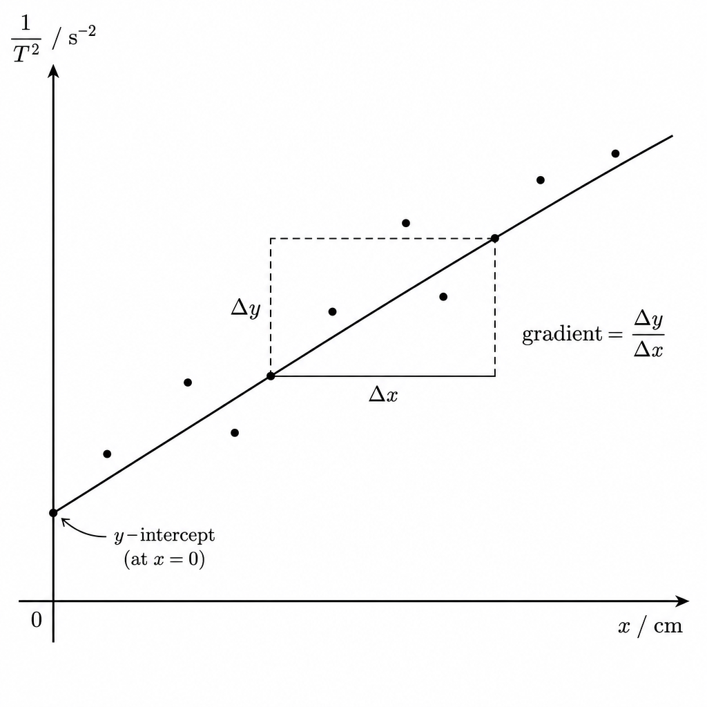
Select two convenient points on the drawn best-fit line (ideally at grid intersections).
Read their coordinates carefully using the axis scales.
Calculate

\Delta y = y_2 - y_1, \quad \Delta x = x_2 - x_1

then

\text{gradient} = \frac{\Delta y}{\Delta x}.

Determine the $y$ -intercept:

either read directly at $x=0$ , or
use

q = y - (\text{gradient})x

with a point $(x,y)$ on the line.

Using the illustrative points $(15.0,0.65)$ and $(40.0,1.40)$ :

\text{gradient} = \frac{1.40 - 0.65}{40.0 - 15.0} = 3.00\times 10^{-2}\ \text{s}^{-2}\ \text{cm}^{-1}

and

q = 0.65 - (3.00\times 10^{-2})(15.0) = 0.20\ \text{s}^{-2}.

Key Takeaways

Use the best-fit line, not point-to-point values.
Use a large triangle for better accuracy.
Units of gradient come from (units of $y$ )/(units of $x$ ).

Common Mistakes

Calculating gradient as $\Delta x/\Delta y$ .
Using two plotted points that are close together.
Using two raw data points instead of points on the best-fit line.
Writing the intercept with the wrong units (it must match $y$ units).

Things to Be Careful About

Read values from the drawn line, not from the table, when finding gradient/intercept.
Keep consistent units: if $x$ is in cm on the graph, gradient must be per cm (not per m).
Quote sensible significant figures (typically 2–3 s.f. depending on graph reading precision).

Techniques used

use a large triangle on the best-fit line to calculate the gradientcalculate gradient as $\Delta y / \Delta x$read the y-intercept from the graph at $x = 0$

(e)

The quantities $x$ and $T$ are related by the equation

\frac{1}{T^2} = px + q

where $p$ and $q$ are constants.

Use your answers from (d)(iii) to determine the values of $p$ and $q$ .
Give appropriate units.

$p$ = ______
$q$ = ______

DifficultyMedium-Easy

Worked solution

Working

Given

\frac{1}{T^2} = px + q

Comparing with $y = mx + c$ for a graph of $y = 1/T^2$ against $x$ :

p = \text{gradient}, \quad q = y\text{-intercept}

Units:

$q$ has units of $1/T^2$ : $\text{s}^{-2}$ .
$p$ has units of $(\text{s}^{-2})/(\text{cm}) = \text{s}^{-2}\ \text{cm}^{-1}$ (if $x$ plotted in cm).

Answer

$p = 3.00\times 10^{-2}\ \text{s}^{-2}\ \text{cm}^{-1}$

$q = 0.20\ \text{s}^{-2}$

Final answer

p = 3.00×10^-2 s^-2 cm^-1, q = 0.20 s^-2

Detailed explanation

Background Concept

If two variables obey a linear relationship

y = mx + c,

a graph of $y$ against $x$ is a straight line with:

gradient $m$ ,
$y$ -intercept $c$ .

Here, the given model is

\frac{1}{T^2} = px + q.

This is already in straight-line form with $y = 1/T^2$ and $x = x$ .

Understanding the Question

You have already plotted $1/T^2$ (vertical) against $x$ (horizontal) and found the gradient and intercept. You are now asked to use those graph values to determine the constants $p$ and $q$ , including their units.

Approach

Match the equation to $y = mx + c$ :

$p$ corresponds to the gradient,
$q$ corresponds to the intercept.
Then assign units based on the axes units.

Step-by-Step Reasoning

Identify plotted variables:
- $y = 1/T^2$ with units $\text{s}^{-2}$ ,
- $x$ with units from your graph (often $\text{cm}$ ).
Compare with $y = mx + c$ :

\frac{1}{T^2} = px + q \quad \Rightarrow \quad p = m,\ q = c.

Units:

Since $q$ is added directly to $px$ to give $1/T^2$ , it must have the same units as $1/T^2$ :

[q] = \text{s}^{-2}.

For $px$ to have units $\text{s}^{-2}$ , the unit of $p$ must be

[p] = \frac{\text{s}^{-2}}{\text{cm}} = \text{s}^{-2}\ \text{cm}^{-1}

(if $x$ is plotted in cm; if plotted in m then $[p] = \text{s}^{-2}\ \text{m}^{-1}$ ).

Substitute your numerical gradient and intercept from (d)(iii) to obtain $p$ and $q$ .

Key Takeaways

When the equation is already linear, the graph directly gives constants.
Always derive units from the axes.

Common Mistakes

Swapping $p$ and $q$ .
Giving $q$ the wrong units (it must be $\text{s}^{-2}$ ).
Converting $x$ to metres for units without actually plotting $x$ in metres.

Things to Be Careful About

Use the same unit for $x$ that you used on the graph when stating units of $p$ .
Quote $p$ and $q$ to a sensible number of significant figures consistent with graph-reading uncertainty.

Techniques used

match a linear equation to y = mx + cidentify constants from gradient and interceptdeduce units of constants from the plotted variables

The rest of this paper

1 more questions

Q2Manipulation, Measurement and Observation · Presentation of Data and Observations · Analysis, Conclusions and Evaluation20M

Loading the full paper…