Physics 9702/33 — October/November 2015

Cambridge AS Level · Advanced Practical Skills · worked solutions for every part, with the mark scheme

questions

marks

120

minutes

Topics Manipulation, Measurement and Observation · Presentation of Data and Observations · Analysis, Conclusions and Evaluation

Q1Manipulation, Measurement and ObservationPresentation of Data and ObservationsAnalysis, Conclusions and EvaluationFree sample

In this experiment, you will investigate the equilibrium of a wooden rod.

(a)

Set up the apparatus as shown in Fig. 1.1.

Fig. 1.1

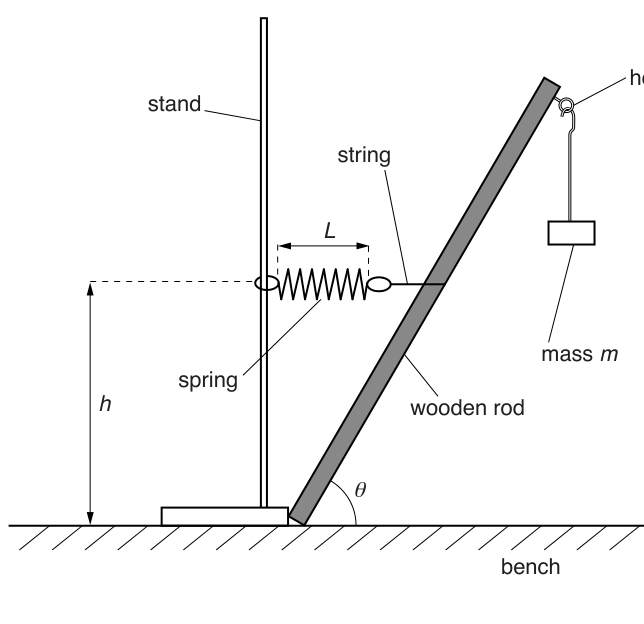
The mass $m$ should be $60\text{ g}$ . The string should be approximately half-way along the wooden rod. The spring should be horizontal.

DifficultyMedium-Easy

Worked solution

Answer

Set up the rod, spring and string as in Fig. 1.1 with $m = 60\ \text{g}$ .

Adjust so that:

the string is attached approximately halfway along the rod,
the spring is horizontal,
the rod is in equilibrium (steady, not slipping).

Final answer

See working

Detailed explanation

Background Concept

This is an equilibrium practical: the rod is at rest, so it has no resultant force and no resultant moment (turning effect). For the measurements later to be meaningful, the apparatus must match the diagram and be in a steady equilibrium position.

Key practical ideas:

Alignment matters: “spring horizontal” and “string horizontal” are geometric conditions that affect the relationship you will test.
Repeatability depends on a stable set-up: if the rod slips, or the spring is not at the stated position, the readings of $h$ and $\theta$ will change.

Understanding the Question

You are instructed to set up the apparatus exactly as shown:

a wooden rod rests against the bench making an angle $\theta$ with the bench,
a horizontal spring is attached to the rod and to a clamp stand,
a string is attached to the rod, passes over a hook at the top region, and supports a mass $m$ ,
initially $m$ should be $60\ \text{g}$ and the string should be about halfway along the rod.

This part is about getting a correct, workable set-up ready for accurate measurements in later parts.

Approach

Assemble the hardware (bench, rod, clamp stand, spring, string, mass hanger).
Set $m = 60\ \text{g}$ .
Adjust the attachment point of the string to be roughly halfway along the rod.
Adjust the clamp stand height/position so that the spring is horizontal.
Ensure the rod is steady and does not slip before taking any measurements.

Step-by-Step Reasoning

diagram-1a

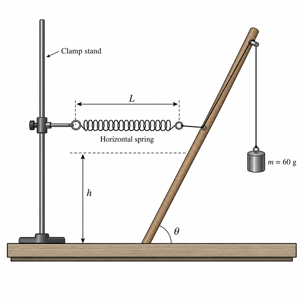
Place one end of the wooden rod on the bench and lean it so it makes a clear angle with the bench surface.
Attach the spring between the rod and the clamp stand.
Move the clamp stand (or change clamp height) until the spring is visibly horizontal (use the bench edge as a reference line).
Tie/attach the string to the rod at approximately the midpoint of the rod (halfway along its length), then route it over the hook as shown and attach the mass hanger.
Add masses until the total hanging mass is $60\ \text{g}$ .
Check that the rod and attachments are in equilibrium: no motion, no slipping at the contact point with the bench, and the spring and string remain taut.

Key Takeaways

Correct set-up is essential: later calculations assume the spring/string are horizontal when stated.
A stable equilibrium position improves accuracy and repeatability.

Common Mistakes

Spring not actually horizontal (introduces systematic error in $h$ and the geometry).
String not positioned roughly halfway along the rod (changes the torque balance and alters results).
Rod slipping during readings (gives inconsistent $h$ and $\theta$ ).

Things to Be Careful About

Ensure the mass value is the total hanging mass ( $60\ \text{g}$ including any hanger if required by your lab’s convention).
Ensure the spring is horizontal at the moment you take readings (not just “about horizontal”).
Keep the bench contact point consistent; if the rod base moves, your geometry changes.

Techniques used

assemble apparatus to match a given diagramadjust the spring to be horizontalposition the string approximately halfway along the rodhang the specified mass securely and check equilibrium

(b)

(i)

Measure and record the length $L$ of the coiled part of the spring.

$L$ = ______

DifficultyEasy

Worked solution

Answer

Measure the coiled length of the spring with a ruler.

Example: $L = 6.2\ \text{cm}$ (to the nearest $0.1\ \text{cm}$ ).

Final answer

L = 6.2 cm

Detailed explanation

Background Concept

A length measurement should be:

taken with an appropriate instrument (typically a mm-scale ruler),
recorded to a precision consistent with the scale (usually to the nearest mm, i.e. $0.1\ \text{cm}$ ),
clearly defined: here, the question specifies the coiled part of the spring, so you must not include any straight end hooks or connecting loops unless they are part of the coiled region.

Understanding the Question

You must measure $L$ , the length of the coiled part of the spring, while the apparatus is set up (with $m = 60\ \text{g}$ in part (a)). The value of $L$ will later be kept constant for different masses, so this initial measurement is important.

Approach

Identify the start and end of the coiled section.
Align a ruler parallel to the spring.
Read $L$ at eye level to reduce parallax.
Record $L$ with a unit and appropriate precision.

Step-by-Step Reasoning

Place the ruler alongside the spring so that the ruler’s zero is aligned with one end of the coiled section.
Read the position of the other end of the coiled section.
Subtract if the zero cannot be aligned exactly.
Record in cm to $0.1\ \text{cm}$ (or in mm to $1\ \text{mm}$ ).

Example recording:

L = 6.2\ \text{cm}

Key Takeaways

Measure the correct feature (coiled part only).
Record to appropriate resolution with units.

Common Mistakes

Measuring the entire spring including loops/hooks.
Reading from an angle (parallax error).
Writing a value with inappropriate precision (e.g. $6\ \text{cm}$ when a mm scale was used).

Things to Be Careful About

Keep the spring straight and horizontal while measuring.
If the spring is slightly stretched, ensure you still measure the coiled section end-to-end consistently in each trial.

Techniques used

measure a length with a ruler to the appropriate precisionidentify and measure only the coiled portion of the springrecord a reading with consistent units and appropriate decimal places

(ii)

Measure and record the height $h$ of the loop of the spring above the bench.

$h$ = ______

DifficultyMedium-Easy

Worked solution

Answer

Measure the vertical height of the spring loop above the bench.

Example: $h = 10.5\ \text{cm}$ (to the nearest $0.1\ \text{cm}$ ).

Final answer

h = 10.5 cm

Detailed explanation

Background Concept

A height $h$ is a vertical distance from a reference level (here, the bench surface). If you measure along a slanted line, you do not get the true height. In practical work, a set square (or measuring from a vertical ruler) helps ensure the measurement is vertical.

Understanding the Question

You must measure $h$ , defined as the height of the loop (attachment point) of the spring above the bench.

Reference: the bench surface.
Point: the spring loop/attachment point at the rod.

Approach

Use a ruler (or metre rule) held vertically with its zero at the bench surface.
Ensure the reading is taken at the level of the loop using a set square (horizontal sight line).

Step-by-Step Reasoning

Position a metre rule vertically with its zero on the bench.
Bring a set square (or another ruler) horizontally from the spring loop to meet the vertical scale.
Read the vertical scale at the intersection.
Record to the nearest mm (or $0.1\ \text{cm}$ ).

Example:

h = 10.5\ \text{cm}

Key Takeaways

Heights must be measured vertically from the correct reference surface.
Use alignment aids to reduce parallax and angular errors.

Common Mistakes

Measuring from the floor instead of from the bench.
Measuring along the rod/spring instead of vertically.
Guessing the height without aligning to the loop level.

Things to Be Careful About

Take the reading at eye level to avoid parallax.
Make sure you measure the height of the loop (exact point specified), not the clamp or a different part of the spring.

Techniques used

measure a vertical height relative to a reference surfaceuse a set square or plumb line to ensure a vertical measurementrecord a measurement with appropriate precision and unit

(iii)

Measure and record the angle $\theta$ between the wooden rod and the bench.

$\theta$ = ______ $^{\circ}$

DifficultyMedium-Easy

Worked solution

Answer

Measure the angle between the rod and the bench using a protractor.

Example: $\theta = 52^{\circ}$ .

Final answer

θ = 52°

Detailed explanation

Background Concept

An angle measurement is only meaningful if you measure the angle between the correct two straight lines.
Here, $\theta$ is the angle between the rod and the bench:

one line is along the rod,
the other is along the bench surface (a horizontal line).

Understanding the Question

You must record $\theta$ in degrees. This angle will be used later in calculating $\cos\theta$ , so a reasonable precision (typically nearest degree) is expected.

Approach

Use a protractor.
Align the protractor’s baseline with the bench (horizontal).
Align the centre at the contact point (or use an extended straight edge along the rod).
Read where the rod line crosses the protractor scale.

Step-by-Step Reasoning

Place a straight edge along the rod to define a clear line.
Place the protractor with its origin at the rod’s base point on the bench.
Ensure the $0^{\circ}$ line is parallel to the bench.
Read the angle up to the rod line.

Example:

\theta = 52^{\circ}

Key Takeaways

Angles depend on correct alignment; small misalignment can change $\cos\theta$ noticeably.

Common Mistakes

Measuring the complementary angle (e.g. between rod and vertical rather than rod and horizontal).
Not aligning the baseline with the bench.
Reading the wrong protractor scale (inner vs outer).

Things to Be Careful About

Keep the rod steady while reading.
Record as an integer number of degrees unless your protractor clearly supports half-degrees.

Techniques used

measure an angle using a protractoridentify the correct angle between two lines/surfacesrecord an angle to a sensible precision

(c)

Change mass $m$ to $80\text{ g}$ .

Adjust the position of the spring and string so that the length $L$ is the same as in (b)(i) and the string is horizontal.

Repeat (b)(ii) and (b)(iii).

$h$ = ______
$\theta$ = ______ $^{\circ}$

DifficultyMedium

Worked solution

Answer

Change to $m = 80\ \text{g}$ . Adjust spring and string so that $L$ is the same as in (b)(i) and the string is horizontal.

Example readings:

h = 11.7\ \text{cm}

\theta = 56^{\circ}

Final answer

h = 11.7 cm, θ = 56°

Detailed explanation

Background Concept

In practical investigations, you often vary one quantity (here $m$ ) while keeping another fixed (here the spring’s coiled length $L$ ). This control is vital so that any change in the measured geometry ( $h$ and $\theta$ ) is due to the intended change in $m$ , not because the spring extension changed.

Also, the instruction “string is horizontal” defines a specific geometry; if the string slopes, you introduce a systematic error because the forces/geometry are no longer the intended ones.

Understanding the Question

You must:

Change the mass from $60\ \text{g}$ to $80\ \text{g}$ .
Adjust the apparatus so that:

$L$ stays the same as your earlier value,
the string is horizontal.

Measure and record new values of $h$ and $\theta$ .

Approach

Replace the mass.
Adjust the clamp stand position/height and the string attachment point until the spring returns to the same coiled length $L$ as in (b)(i).
Check the string is horizontal (use a ruler/bench edge for reference).
Then measure $h$ and $\theta$ using the same methods as in (b)(ii) and (b)(iii).

Step-by-Step Reasoning

Add masses to make $m = 80\ \text{g}$ .
Observe that the geometry changes; the spring length will generally change.
Move the spring attachment/clamp stand so that the coiled length matches your recorded $L$ (measure and adjust until it agrees).
Adjust the string attachment so the string is horizontal (compare against a horizontal reference line).
Once stable, measure:
- $h$ as a vertical height above the bench,
- $\theta$ as the angle between rod and bench.

Example set of readings:

h = 11.7\ \text{cm}

\theta = 56^{\circ}

Key Takeaways

This is controlled variation: change $m$ , keep $L$ fixed.
Always re-check alignment conditions (horizontal spring/string) before reading instruments.

Common Mistakes

Forgetting to reset $L$ to the original value.
Taking readings before the string is properly horizontal.
Measuring $h$ from the wrong reference (not the bench).

Things to Be Careful About

Re-measure $L$ after adjustments; do not rely on appearance.
Ensure the apparatus is not oscillating when you read $h$ and $\theta$ .

Techniques used

change the load while keeping another variable constantadjust apparatus to maintain a fixed spring lengthensure the string is horizontal before taking readingsrepeat measurements consistently

(d)

(i)

Copy your value of $L$ from (b)(i).

$L$ = ______

DifficultyEasy

Worked solution

Answer

Copied from (b)(i):

Example: $L = 6.2\ \text{cm}$ .

Final answer

L = 6.2 cm

Detailed explanation

Background Concept

In many practicals a measured quantity is used as a control variable. Writing it again reduces the chance of accidentally using a different value later.

Understanding the Question

You are told to copy your previously measured $L$ (coiled spring length) so you can use it as the fixed value while collecting multiple data sets in (d)(ii).

Approach

Simply transfer the value exactly as recorded in (b)(i), keeping the same unit and precision.

Step-by-Step Reasoning

If your (b)(i) reading was, for example,

L = 6.2\ \text{cm}

then write the same here.

Key Takeaways

Consistency of the control variable is essential for valid results.

Common Mistakes

Changing the number of decimal places or unit when copying.
Copying the wrong length (e.g. total spring length instead of coiled length).

Things to Be Careful About

Keep $L$ exactly the same during later adjustments; this copied value is the target each time.

Techniques used

transfer a recorded measurement consistentlyuse a fixed reference value for controlled experiments

(ii)

Change $m$ and repeat (b)(ii) and (b)(iii) until you have six sets of values of $m$ , $h$ and $\theta$ .
For each value of $m$ , adjust the position of the spring and string so that $L$ is the same as in (d)(i) and the spring is horizontal.

Include your values from (b) and (c).

Also include values of $\frac{h}{\cos \theta}$ in your table.

10M

DifficultyMedium

Worked solution

Answer

Take six sets of readings of $m$ , $h$ and $\theta$ (including the $60\ \text{g}$ and $80\ \text{g}$ cases), keeping $L$ constant and the spring horizontal each time.

Record all results in one table with headings and units, and calculate $\dfrac{h}{\cos\theta}$ for each set.

Example (illustrative):

$m / \text{g}$	$h / \text{cm}$	$\theta / ^\circ$	$\dfrac{h}{\cos\theta} / \text{cm}$
40	8.7	48	13.0
50	9.6	50	15.0
60	10.5	52	17.0
70	11.2	54	19.0
80	11.7	56	21.0
90	12.2	58	23.0

Final answer

See working

Detailed explanation

Background Concept

A good data table in Paper 3 is assessed on:

Sufficient data: at least six sets over a sensible range of the independent variable.
Clear headings: each column labelled with the quantity and unit, e.g. $h / \text{cm}$ .
Consistent precision: similar decimal places/precision within a column.
Correct calculated quantities: derived values computed correctly from the measured values.

Here you are also told to calculate:

\frac{h}{\cos\theta}

Since $\cos\theta$ is dimensionless, $h/\cos\theta$ has the same unit as $h$ .

Understanding the Question

You must build a table containing six sets of:

$m$ (changed each run),
$h$ (measured),
$\theta$ (measured),
and the calculated quantity $h/\cos\theta$ .

For each new $m$ you must adjust the apparatus so that:

$L$ is the same as in (d)(i),
the spring is horizontal.
You must include your earlier results from (b) and (c).

Approach

Choose six values of $m$ spanning a reasonable range (including $60\ \text{g}$ and $80\ \text{g}$ ).
For each $m$ $m$ :
- adjust until $L$ matches the fixed value,
- check spring horizontal,
- measure $h$ and $\theta$ .
Calculate $h/\cos\theta$ for each row.
Present everything in one neat table with units and consistent precision.

Step-by-Step Reasoning

Pick masses such as $40, 50, 60, 70, 80, 90\ \text{g}$ (any sensible range with six values is acceptable).
For each mass:
- ensure the spring coiled length equals your fixed $L$ value (re-measure $L$ to confirm),
- measure $h$ vertically from the bench,
- measure $\theta$ between rod and bench.
Compute $h/\cos\theta$ $h / cos θ$ :
- calculate $\cos\theta$ (calculator in degree mode),
- divide $h$ by $\cos\theta$ .

Example calculation for one row (illustrative): if $h = 10.5\ \text{cm}$ and $\theta = 52^{\circ}$ ,

\cos 52^{\circ} \approx 0.616

\frac{h}{\cos\theta} = \frac{10.5}{0.616} \approx 17.0\ \text{cm}

Key Takeaways

Use enough readings and a good range of $m$ .
Keep control variables constant ( $L$ and spring horizontal) to make the test valid.
Present raw and derived data clearly with units and consistent precision.

Common Mistakes

Fewer than six sets of results.
Missing units in headings (e.g. writing just $m$ instead of $m / \text{g}$ ).
Inconsistent decimal places (e.g. mixing $10.5\ \text{cm}$ and $10.53\ \text{cm}$ without reason).
Calculating $h\cos\theta$ instead of $h/\cos\theta$ .

Things to Be Careful About

Ensure calculator is in degrees for $\cos\theta$ .
Quote $h/\cos\theta$ to a sensible number of significant figures (usually matching $h$ ).
Do not change $L$ between runs; this is a key control.

Techniques used

select a suitable range and number of values for the independent variablerecord raw measurements in a structured table with unitscalculate a derived quantity from measured valuesuse consistent significant figures within each column

(e)

(i)

Plot a graph of $\frac{h}{\cos \theta}$ on the $y$ -axis against $m$ on the $x$ -axis.

DifficultyMedium-Easy

Worked solution

Answer

Plot $\dfrac{h}{\cos\theta}$ (y-axis) against $m$ (x-axis).

Axes labels (example):

$x$ -axis: $m / \text{g}$
$y$ -axis: $\dfrac{h}{\cos\theta} / \text{cm}$

Use a suitable scale and plot all six points accurately.

Final answer

See working

Detailed explanation

Background Concept

A good physics graph should:

have correctly labelled axes with units,
use a sensible scale (not cramped; typically use at least half the grid in each direction),
have accurately plotted points (fine pencil, small crosses or dots),
match the instruction for which quantity goes on which axis.

Understanding the Question

You are told exactly what to plot:

vertical axis: $\dfrac{h}{\cos\theta}$ ,
horizontal axis: $m$ .
You should use your calculated values from the table in (d)(ii).

Approach

Decide the range of $m$ and $h/\cos\theta$ from your table.
Choose convenient scales (e.g. 10 g per large square; 2 cm per large square, etc.) that spread the data.
Label each axis with both the symbol/expression and its unit.
Plot each point carefully.

Step-by-Step Reasoning

Mark axes and label:
- $m / \text{g}$ or $m / \text{kg}$ (depending on what you used in the table),
- $\dfrac{h}{\cos\theta} / \text{cm}$ (or / m).
Choose scales so the smallest and largest values fit with good spread.
Plot the six points from your table.

Key Takeaways

Correct graph choice and correct axis labelling are easy marks.
Using the full grid improves accuracy when finding gradient and intercept.

Common Mistakes

Swapping axes (plotting $m$ on the y-axis).
Missing units or writing units incorrectly in the labels.
Using an awkward scale (e.g. 3 g per square) that makes plotting error-prone.

Things to Be Careful About

Plot $h/\cos\theta$ , not just $h$ .
Keep consistent units: if $h$ is in cm, then $h/\cos\theta$ is also in cm.

Techniques used

choose suitable axis scales to use most of the gridlabel axes with quantity and unitplot points accurately from a results table

(ii)

Draw the straight line of best fit.

DifficultyMedium-Easy

Worked solution

Answer

Draw a single straight line of best fit through the plotted points (not point-to-point).

Final answer

See working

Detailed explanation

Background Concept

A best-fit line represents the overall trend in the data. For experimental results there will be scatter, so the best-fit line should be positioned so that the points are approximately balanced above and below the line.

Understanding the Question

You have plotted $\dfrac{h}{\cos\theta}$ against $m$ . You must now draw the straight line of best fit.

Approach

Use a ruler.
Draw one straight line that follows the trend.
Ensure it is not forced through every point or through the origin unless the data clearly supports it.

Step-by-Step Reasoning

Visually assess the general linear trend.
Place a ruler so that there are roughly equal numbers of points above and below the line (and similar average distances).
Draw a thin, continuous straight line across the whole data range.

Key Takeaways

Best-fit is not “join-the-dots”.
Do not assume the line must pass through $(0,0)$ .

Common Mistakes

Connecting points with zig-zag segments.
Forcing the line through an outlier.
Forcing the line through the origin without evidence.

Things to Be Careful About

Extend the line far enough to allow a reliable intercept reading.
Keep the line thin so that gradient/intercept readings are not ambiguous.

Techniques used

draw a single straight line of best fit through plotted pointsbalance deviations so points lie roughly evenly around the line

(iii)

Determine the gradient and $y$ -intercept of this line.

gradient = ______
$y$ -intercept = ______

DifficultyMedium-Easy

Worked solution

Working

Using two points on the best-fit line, e.g. $(m, y) = (40\ \text{g}, 13.0\ \text{cm})$ and $(90\ \text{g}, 23.0\ \text{cm})$ :

\text{gradient} = \frac{\Delta y}{\Delta x} = \frac{23.0 - 13.0}{90 - 40} = \frac{10.0}{50} = 0.20\ \text{cm g}^{-1}

$y$ -intercept at $m = 0$ :

y = 5.0\ \text{cm}

Answer

gradient $= 0.20\ \text{cm g}^{-1}$

$y$ -intercept $= 5.0\ \text{cm}$

Final answer

gradient = 0.20 cm g^-1, y-intercept = 5.0 cm

Detailed explanation

Background Concept

For a straight-line graph, the gradient and y-intercept describe the line:

Gradient:

\text{gradient} = \frac{\Delta y}{\Delta x}

y-intercept: the value of $y$ when $x = 0$ .

In practical graphs, you should use two points on the best-fit line, not necessarily two experimental points, and choose them far apart to reduce percentage reading uncertainty.

Understanding the Question

You must extract two values from your straight line:

the gradient,
the y-intercept.
These will be used in part (f) to determine constants $A$ and $B$ .

Approach

Pick two widely separated points on the drawn best-fit line (read their coordinates).
Compute gradient using $\Delta y/\Delta x$ .
Read the y-intercept by extending the best-fit line to $m = 0$ and reading $y$ .
Include correct units.

Step-by-Step Reasoning

Choose two points on the line far apart.
Read coordinates carefully, matching the axis scales.
Calculate:

\text{gradient} = \frac{y_2 - y_1}{m_2 - m_1}

Determine intercept by reading where the line crosses the y-axis.

Illustrative example (your values depend on your graph):

\text{gradient} = \frac{23.0 - 13.0}{90 - 40} = 0.20\ \text{cm g}^{-1}

\text{y-intercept} = 5.0\ \text{cm}

Key Takeaways

Use points on the best-fit line and make the triangle large.
Gradient is always “change in y divided by change in x”.
Include units: gradient has units of (y-units)/(x-units).

Common Mistakes

Using two nearby points, giving a large percentage uncertainty.
Swapping $\Delta x$ and $\Delta y$ (calculating $\Delta x/\Delta y$ ).
Using two data points that are not on the best-fit line.
Forgetting units, or using inconsistent units (e.g. $m$ in g but quoting gradient per kg).

Things to Be Careful About

If your axes are $m / \text{kg}$ and $y / \text{m}$ then your units will change (e.g. gradient in $\text{m kg}^{-1}$ ).
Read intercept from the best-fit line extended to the y-axis, not from the first plotted point.

Techniques used

select two widely separated points on a best-fit linecalculate the gradient as $\Delta y / \Delta x$read the y-intercept at $x = 0$

(f)

The quantities $h$ , $\theta$ and $m$ are related by the equation

\frac{h}{\cos \theta} = Am + B

where $A$ and $B$ are constants.

Using your answers in (e)(iii), determine the values of $A$ and $B$ .
Give appropriate units.

$A$ = ______
$B$ = ______

DifficultyMedium-Easy

Worked solution

Working

Given

\frac{h}{\cos\theta} = Am + B

Comparing with $y = mx + c$ for a graph of $y = \dfrac{h}{\cos\theta}$ against $x = m$ :

A = \text{gradient}, \qquad B = \text{y-intercept}

Using (e)(iii):

A = 0.20\ \text{cm g}^{-1}

B = 5.0\ \text{cm}

Answer

$A = 0.20\ \text{cm g}^{-1}$

$B = 5.0\ \text{cm}$

Final answer

A = 0.20 cm g^-1, B = 5.0 cm

Detailed explanation

Background Concept

If a relationship is linear:

y = mx + c

then a graph of $y$ against $x$ is a straight line with:

gradient $m$ ,
y-intercept $c$ .

Here,

\frac{h}{\cos\theta} = Am + B

This is already in linear form if you treat $\dfrac{h}{\cos\theta}$ as $y$ and $m$ as $x$ .

Units:

$h/\cos\theta$ has the same unit as $h$ (since $\cos\theta$ is dimensionless).
Therefore $B$ has the same unit as $h$ .
$A$ has units:

[A] = \frac{[h]}{[m]}

So if $h$ is in cm and $m$ is in g, then $A$ is in $\text{cm g}^{-1}$ .

Understanding the Question

You are asked to determine $A$ and $B$ using your gradient and y-intercept from (e)(iii), and to include appropriate units.

Approach

Recognise that the plotted graph is exactly $y$ vs $x$ for the linear equation.
Set $A =$ gradient and $B =$ y-intercept.
Assign units from the graph axes.

Step-by-Step Reasoning

From the instruction in (e)(i), the graph is:

$y$ -axis: $y = \dfrac{h}{\cos\theta}$
$x$ -axis: $x = m$
So the equation becomes:

y = Ax + B

Therefore:

A = \text{gradient of the best-fit line}

B = \text{y-intercept of the best-fit line}

Using example values from (e)(iii):

A = 0.20\ \text{cm g}^{-1}

B = 5.0\ \text{cm}

Key Takeaways

When the equation is already linear, constants come directly from gradient and intercept.
Units come from the axes: gradient has units (y-units)/(x-units).

Common Mistakes

Swapping $A$ and $B$ .
Giving no units.
Using inconsistent units (e.g. graph plotted with $m$ in g but quoting $A$ in $\text{m kg}^{-1}$ ).

Things to Be Careful About

If you plotted $m$ in kg instead of g, your numerical value for $A$ would change by a factor of $1000$ .
Quote $A$ and $B$ to a reasonable number of significant figures consistent with your graph reading accuracy.

Techniques used

match a linear equation to $y = mx + c$identify constants from gradient and interceptdeduce units of constants from axis units

The rest of this paper

1 more questions

Q2Manipulation, Measurement and Observation · Presentation of Data and Observations · Analysis, Conclusions and Evaluation20M

Loading the full paper…