Physics 9702/35 — October/November 2014

Cambridge AS Level · Advanced Practical Skills · worked solutions for every part, with the mark scheme

questions

marks

120

minutes

Topics Manipulation, Measurement and Observation · Presentation of Data and Observations · Analysis, Conclusions and Evaluation

Q1Manipulation, Measurement and ObservationPresentation of Data and ObservationsAnalysis, Conclusions and EvaluationFree sample

In this experiment, you will investigate the motion of masses suspended from springs.

(a)

(i)

Set up the apparatus as shown in Fig. 1.1.

Fig. 1.1

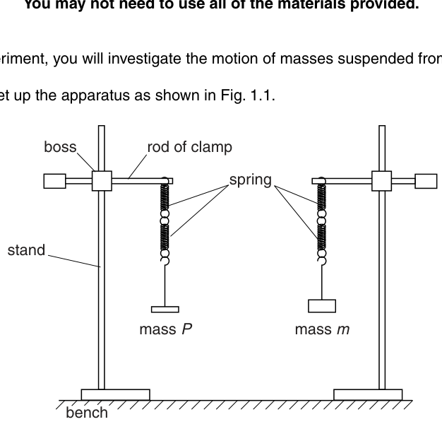
The mass $P$ must be $200\text{ g}$ and must remain constant throughout the experiment.
The mass $m$ should be $250\text{ g}$ .

DifficultyEasy

Worked solution

Answer

Set up two springs on separate clamp stands as in Fig. 1.1.
Attach mass $P = 200\ \text{g}$ to the left spring and keep $P$ constant throughout.
Attach mass $m = 250\ \text{g}$ to the right spring.

Final answer

Apparatus set up with P = 200 g constant and m = 250 g.

Detailed explanation

Background Concept

In oscillation experiments, the main practical requirements are that the mass can move freely in a vertical line and that the spring is not rubbing against the stand or twisting significantly. If the motion is not vertical or the spring touches the stand, the motion becomes irregular and timing becomes unreliable.

Understanding the Question

You are told to build the apparatus exactly as in Fig. 1.1 with two springs and two hanging masses. The key instruction is that $P$ must be $200\ \text{g}$ and must not be changed during the experiment, while $m$ starts at $250\ \text{g}$ and will be varied later.

Approach

Clamp the supports securely so they do not move.
Hang one spring from each clamp.
Attach the specified masses.
Ensure both masses have clearance to oscillate vertically.

Step-by-Step Reasoning

diagram-1

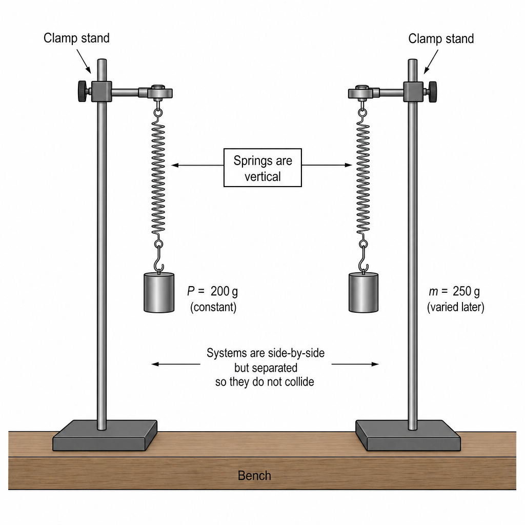
Use two stands so that each spring–mass system is independent.
Hang each spring from a clamp so the spring is vertical.
Attach mass $P$ to one spring and set $P = 200\ \text{g}$ .
Attach mass $m$ to the other spring and set $m = 250\ \text{g}$ .
Check that, when displaced, neither mass hits the bench or stand and the springs do not collide.

Key Takeaways

Good oscillation timing depends on smooth, vertical motion.
Keeping $P$ constant is essential because the experiment investigates how the behaviour changes as $m$ is changed.

Common Mistakes

Changing $P$ during the experiment.
Allowing the mass to swing sideways (pendulum motion) instead of oscillating vertically.
Setting the stands too close so the masses/springs interfere.

Things to Be Careful About

Ensure clamps are tight and the stand does not topple.
Ensure the mass hanger is secure so it cannot fall.
Keep the initial displacements small so the oscillations are approximately simple harmonic and repeatable.

Techniques used

assemble the apparatus as shown in the diagramensure the specified mass is kept constantcheck alignment so the masses oscillate freely without touching the stand

(ii)

Calculate and record $(m - P)$ .

$(m - P)$ = ______

DifficultyEasy

Worked solution

Working

(m-P) = 250\ \text{g} - 200\ \text{g} = 50\ \text{g}

Answer

$(m-P) = 50\ \text{g}$ ( $= 0.050\ \text{kg}$ )

Final answer

50 g (0.050 kg)

Detailed explanation

Background Concept

When two masses are given in the same units, their difference is found by simple subtraction. In practical work you should record calculated quantities clearly with units. Later analysis (especially gradients) is often easier if masses are in SI units (kg).

Understanding the Question

You have $m = 250\ \text{g}$ and $P = 200\ \text{g}$ . You are asked to calculate $(m-P)$ and record it.

Approach

Subtract $P$ from $m$ in grams (since both are given in grams). Optionally convert to kilograms for SI use.

Step-by-Step Reasoning

(m-P) = 250\ \text{g} - 200\ \text{g} = 50\ \text{g}

Convert to kg if needed:

50\ \text{g} = 50 \times 10^{-3}\ \text{kg} = 0.050\ \text{kg}

Key Takeaways

Keep units consistent before subtracting.
Record the result with a unit; SI (kg) is often preferred for later graph work.

Common Mistakes

Reversing the subtraction (writing $P-m$ ).
Omitting the unit.
Converting $50\ \text{g}$ to $0.50\ \text{kg}$ (a factor of 10 error).

Things to Be Careful About

Use $1\ \text{g} = 10^{-3}\ \text{kg}$ .
Keep a sensible number of significant figures consistent with the given masses.

Techniques used

calculate a difference between two measured massesconvert grams to kilograms when neededrecord a calculated value with an appropriate unit

(b)

(i)

Pull both masses down through a short distance.
Release both masses at the same time and watch the movement.
The two masses will move up and down becoming out of step.
After a time the masses will be back in step so that they reach the lowest point together.

DifficultyEasy

Worked solution

Answer

After release, the masses oscillate and become out of step (phase difference changes). After some time they are back in step and reach the lowest point together.

Final answer

They go out of step and later return in step, reaching the lowest point together.

Detailed explanation

Background Concept

Two oscillators with slightly different periods gradually develop a changing phase difference: sometimes they move together (in phase) and sometimes one lags behind (out of phase). When the phase difference returns to $0$ (or a whole number of cycles), they are back in step and can reach the same point (e.g. the lowest point) at the same time.

Understanding the Question

You are asked to pull both masses down a short distance, release them together, and watch what happens. The question describes the key observation: the two masses first go out of step, and after some time they come back in step so that they reach the lowest point together.

Approach

Make the initial displacement small and release both masses at the same time to start with approximately the same phase. Then look specifically for the moments when both are at the lowest point at the same instant.

Step-by-Step Reasoning

Displace both masses downward by similar small distances.
Release both simultaneously.
Initially, the motion may appear similar, but because the oscillation periods are not identical, one mass gradually arrives at the lowest point slightly before the other.
The time difference grows until they are clearly out of step.
Continue watching: eventually the faster oscillator “catches up” by one whole cycle relative to the slower, so they again arrive at the lowest point together.

Key Takeaways

“Out of step” means the phase difference is changing.
“Back in step” is a specific repeated event you can use for timing.

Common Mistakes

Allowing sideways swinging, making it hard to judge the lowest point.
Using a large displacement so the motion is less repeatable.
Not releasing simultaneously, so the initial phase is not well-defined.

Things to Be Careful About

Judge the lowest point consistently (same reference event each time).
Avoid touching the masses after release, which can introduce extra motion.

Techniques used

displace both masses by a small amount and release simultaneouslyobserve relative phase between two oscillationsidentify the event when both reach the lowest point together

(ii)

Pull both masses down through a short distance. Release both masses at the same time.
Start the stopwatch when the masses are back in step and reach the lowest point together for the first time.

Measure and record the time $t$ taken for the masses to reach their lowest point together for the sixth time.

$t$ = ______

DifficultyMedium-Easy

Worked solution

Answer

Start timing when both masses first reach the lowest point together after becoming back in step. Stop timing when they reach the lowest point together for the 6th time, and record $t$ (to the nearest $0.1\ \text{s}$ ).

Example: $t = 18.4\ \text{s}$ (student-dependent).

Final answer

t = (student-dependent), e.g. 18.4 s

Detailed explanation

Background Concept

Stopwatch reaction time causes an uncertainty that is roughly constant in absolute terms (e.g. about $\pm 0.2\ \text{s}$ ). To reduce the percentage uncertainty, you time a longer interval by counting multiple repetitions of a clear event, then use that total time.

Understanding the Question

You must:

release both masses;
wait until they are back in step and reach the lowest point together for the first time;
start the stopwatch at that first “together at the lowest point” event;
measure the time for them to reach the lowest point together for the sixth time (i.e. timing five intervals between successive “together” events, depending on counting convention stated).
The instruction explicitly says: start at the first time, measure until the sixth time.

Approach

Use the lowest point together as the single, repeatable reference event. Count occurrences carefully (1st, 2nd, ..., 6th). Record $t$ with appropriate precision (typically $0.1\ \text{s}$ for a digital stopwatch).

Step-by-Step Reasoning

Pull both masses down a small distance and release at the same moment.
Watch until you see them reach the lowest point together for the first time after they have become back in step.
At that instant, start the stopwatch and count it as “1”.
Keep watching and count each subsequent time they reach the lowest point together: “2”, “3”, ...
When you see the 6th time, stop the stopwatch and record the total time $t$ .
Record $t$ to the stopwatch resolution (typically $0.1\ \text{s}$ ).

Key Takeaways

Timing multiple repeats reduces percentage uncertainty.
A consistent event definition is essential for reliable data.

Common Mistakes

Starting timing at the wrong event (e.g. at release rather than at the first in-step lowest point).
Miscounting the occurrences (stopping at the 5th instead of 6th).
Recording too many decimal places that the stopwatch cannot justify.

Things to Be Careful About

Decide your counting clearly: the event you start on is the “first time”, so you stop on the “sixth time” as stated.
Ensure you are judging the lowest point, not just “near the bottom”.
Keep the displacement small to maintain regular oscillations.

Techniques used

time a repeated event over several occurrences to reduce percentage uncertaintyuse a consistent start/stop criterion for stopwatch timingrecord time to an appropriate resolution

(c)

Increase $m$ and repeat (a)(ii) and (b)(ii) until you have six sets of readings of $m$ and $t$ .
Include values of $\frac{1}{t^2}$ and $(m - P)$ in your table.

10M

DifficultyMedium-Hard

Worked solution

Answer

Take six different values of $m$ (with $P = 200\ \text{g}$ constant). For each value:

calculate $(m-P)$
measure $t$ as in (b)(ii)
calculate $\dfrac{1}{t^2}$ .

Record all results in one table with headings including units, e.g.

| $m / \text{kg}$ | $t / \text{s}$ | $(m-P) / \text{kg}$ | $1/t^2 / \text{s}^{-2}$ |

(Values are student-dependent.)

Final answer

Single results table with 6 sets of (m, t) plus calculated (m−P) and 1/t^2.

Detailed explanation

Background Concept

Good experimental data should:

cover a sufficient range of the independent variable (here $m$ ) so any trend is clear;
include enough data points (here six) to justify drawing a best-fit line;
be recorded clearly with units and consistent significant figures;
include calculated columns needed for later graphing (here $(m-P)$ and $1/t^2$ ).

Understanding the Question

You must increase $m$ and repeat the measurement sequence so that you end up with six sets of readings of $m$ and $t$ . You are explicitly told to include $(m-P)$ and $\frac{1}{t^2}$ in your table.

Approach

Choose six values of $m$ that are sensibly spaced.
Keep $P = 200\ \text{g}$ fixed.
For each $m$ , measure $t$ using the same “first-to-sixth lowest point together” rule.
Calculate $(m-P)$ and then compute $1/t^2$ .
Present everything in one clear table with units in the headings.

Step-by-Step Reasoning

Select six values of $m$ (e.g. increasing by equal steps) so that $(m-P)$ spans a useful range.
For each $m$ $m$ :
- record $m$ (preferably in kg for SI);
- calculate $(m-P)$ in kg;
- measure $t$ in seconds;
- calculate $t^2$ and then $1/t^2$ with units $\text{s}^{-2}$ .
Construct a single table:
- each column heading has the quantity and unit;
- raw readings ( $m$ , $t$ ) are recorded to the instrument resolution;
- calculated columns are given to a consistent number of significant figures (typically matching the precision of $t$ ).

Key Takeaways

Six points helps make a reliable graph and best-fit line.
Derived quantities belong in the table because they will be plotted.
Consistent units and significant figures are part of good presentation.

Common Mistakes

Not keeping $P$ constant.
Using too narrow a range of $m$ , producing a weak trend.
Splitting data into multiple tables.
Missing units in headings or mixing grams and kilograms within the same column.
Calculating $1/t$ instead of $1/t^2$ .

Things to Be Careful About

If you use $m$ and $(m-P)$ in grams on the table/graph, your gradient units will be different; SI (kg) is usually safer.
Keep counting of the “sixth time” consistent across all readings.
Use the same number of decimal places for $t$ within a column (consistent resolution).

Techniques used

vary the independent variable over a suitable rangerepeat timing measurements using the same criterioncalculate derived quantities for each readingpresent results in a single table with correct headings and units

(d)

(i)

Plot a graph of $\frac{1}{t^2}$ on the $y$ -axis against $(m - P)$ on the $x$ -axis.

DifficultyMedium

Worked solution

Answer

Plot $y = \dfrac{1}{t^2}$ (unit $\text{s}^{-2}$ ) on the $y$ -axis against $x = (m-P)$ (unit $\text{kg}$ ) on the $x$ -axis, using a suitable scale and plotting all six points accurately.

Final answer

Graph of 1/t^2 (y) against (m−P) (x), with correct labels/units and points plotted.

Detailed explanation

Background Concept

A good physics graph:

has axes labelled with the quantity and unit;
uses a sensible linear scale that uses at least half the available grid;
plots points accurately (small crosses or dots);
does not force the origin unless the data require it.

Understanding the Question

You have calculated $\frac{1}{t^2}$ for each trial and also have $(m-P)$ . You are told exactly what to plot: $\frac{1}{t^2}$ on the vertical axis and $(m-P)$ on the horizontal axis.

Approach

Decide which units you are using for $(m-P)$ (preferably kg).
Choose axis limits to include all your data points.
Pick scales that are easy to plot (e.g. 1 large square = 0.01 in convenient units) and that spread points out.
Plot the six pairs $((m-P),\ 1/t^2)$ .

Step-by-Step Reasoning

From your table, take each value of $(m-P)$ as $x$ and the corresponding $1/t^2$ as $y$ .
Draw axes and label them:
- $x$ -axis: $(m-P) / \text{kg}$ (or / g if you used grams consistently)
- $y$ -axis: $1/t^2 / \text{s}^{-2}$
Choose scales so the plotted points cover a large area of the graph.
Plot each point carefully.

Key Takeaways

The axis choice is part of the assessment: you must plot the specified variables.
Clear labels with units are essential.

Common Mistakes

Swapping axes (plotting $(m-P)$ on $y$ ).
Missing units or writing units incorrectly.
Using an awkward scale (e.g. 3 squares = 0.2) that makes plotting inaccurate.
Plotting $1/t$ instead of $1/t^2$ .

Things to Be Careful About

Ensure you are plotting $1/t^2$ in $\text{s}^{-2}$ , so $t$ must be in seconds.
If you convert masses to kg for the table, be consistent for every point and on the axis label.

Techniques used

choose sensible axis scales that use most of the graph gridlabel axes with quantity and unitplot points accurately from a data table

(ii)

Draw the straight line of best fit.

DifficultyMedium-Easy

Worked solution

Answer

Draw a single straight line of best fit through the plotted points (not point-to-point), with a balanced distribution of points above and below the line.

Final answer

Straight line of best fit drawn.

Detailed explanation

Background Concept

A best-fit line represents the overall trend of the data. Random scatter means not all points lie on a perfect line; the best-fit line should be positioned so the deviations are balanced.

Understanding the Question

After plotting $1/t^2$ against $(m-P)$ , you must draw the straight line that best represents the relationship.

Approach

Use a ruler to draw one straight line that follows the trend and is not forced through every point.

Step-by-Step Reasoning

Place a ruler so that the line passes through the middle of the scatter.
Check there are roughly equal numbers of points (or similar total deviation) above and below.
Draw the line across as much of the graph as possible (long line reduces reading errors later).

Key Takeaways

Do not join consecutive points.
The best-fit line is used to find the gradient and intercept accurately.

Common Mistakes

Drawing a zig-zag line joining points.
Forcing the line through an outlier rather than the overall trend.
Drawing a very short line segment, making gradient readings inaccurate.

Things to Be Careful About

If one point is clearly anomalous, the best-fit line should still reflect the main trend (unless instructed otherwise).
Use a sharp pencil and a ruler for precision.

Techniques used

draw a single straight line that balances points above and belowavoid joining point-to-pointuse the full length of the plotted region for the best-fit line

(iii)

Determine the gradient and $y$ -intercept of this line.

gradient = ______
$y$ -intercept = ______

DifficultyMedium

Worked solution

Working

Choose two points on the best-fit line far apart:

\text{gradient} = \frac{\Delta(1/t^2)}{\Delta(m-P)}

Read $y$ -intercept where $(m-P)=0$ .

(Values are student-dependent.)

Answer

gradient = (from graph)

$y$ -intercept = (from graph)

Final answer

Gradient and y-intercept from best-fit line (student-dependent).

Detailed explanation

Background Concept

For a straight-line graph, the gradient (slope) is

\text{gradient} = \frac{\Delta y}{\Delta x}

and the $y$ -intercept is the value of $y$ when $x=0$ . Using a large triangle on the best-fit line reduces percentage reading uncertainty.

Understanding the Question

You have a graph of $y=1/t^2$ against $x=(m-P)$ . You must find:

the gradient of the best-fit line;
the $y$ -intercept of the best-fit line.

Approach

Pick two widely separated points that lie on the best-fit line (not necessarily your plotted data points).
Read their coordinates accurately from the axes.
Compute $\Delta y$ and $\Delta x$ , then divide.
Extend the best-fit line to meet the $y$ -axis (or read $y$ at $x=0$ ) for the intercept.

Step-by-Step Reasoning

Mark two points on the best-fit line far apart to form a large triangle.
Read coordinates $(x_1,y_1)$ and $(x_2,y_2)$ .
Compute changes:

\Delta y = y_2 - y_1, \qquad \Delta x = x_2 - x_1

Gradient:

\text{gradient} = \frac{\Delta y}{\Delta x}

$y$ -intercept:

either read directly where the line crosses the $y$ -axis;
or set $x=0$ and read the corresponding $y$ value from the line.

Quote units:

if $y$ is in $\text{s}^{-2}$ and $x$ is in $\text{kg}$ , gradient has units $\text{s}^{-2}\ \text{kg}^{-1}$ ;
intercept has units $\text{s}^{-2}$ .

Key Takeaways

Use the best-fit line for gradient/intercept, not a single pair of noisy data points.
A large triangle improves accuracy.

Common Mistakes

Using two neighbouring points, giving a large uncertainty in gradient.
Calculating $\Delta x/\Delta y$ instead of $\Delta y/\Delta x$ .
Using plotted points rather than points on the best-fit line.
Forgetting units.

Things to Be Careful About

Read values from the axes carefully, including powers of ten or scale factors.
Make sure you use consistent units (kg vs g) when interpreting the gradient unit.
Do not round intermediate coordinate readings too aggressively; rounding should be mainly at the final gradient/intercept values.

Techniques used

choose two well-separated points on the best-fit linecalculate gradient using \Delta y / \Delta xread the y-intercept by extrapolating the best-fit line to x = 0

(e)

It is suggested that the quantities $t$ , $m$ and $P$ are related by the equation

\frac{1}{t^2} = U(m - P) + V

where $U$ and $V$ are constants.

Use your answers in (d)(iii) to determine the values of $U$ and $V$ .
Give appropriate units.

$U$ = ______
$V$ = ______

DifficultyMedium-Easy

Worked solution

Working

Given

\frac{1}{t^2} = U(m-P) + V

Comparing with $y = mx + c$ for the graph of $y=1/t^2$ against $x=(m-P)$ :

U = \text{gradient}, \qquad V = y\text{-intercept}

Units (if $(m-P)$ in kg):

[U] = \frac{\text{s}^{-2}}{\text{kg}} = \text{s}^{-2}\ \text{kg}^{-1}, \qquad [V] = \text{s}^{-2}

Answer

$U$ = gradient (from (d)(iii)) in $\text{s}^{-2}\ \text{kg}^{-1}$

$V$ = $y$ -intercept (from (d)(iii)) in $\text{s}^{-2}$

Final answer

U = gradient (s^-2 kg^-1); V = y-intercept (s^-2)

Detailed explanation

Background Concept

A straight-line relationship has the form

y = mx + c

where $m$ is the gradient and $c$ is the $y$ -intercept. If you plot the correct variables on the axes, you can read off constants in the equation directly:

gradient corresponds to the coefficient of $x$ ;
intercept corresponds to the constant term.
Units come from the plotted quantities:

[m] = \frac{\text{units of } y}{\text{units of } x}, \qquad [c] = \text{units of } y.

Understanding the Question

You are told the suggested relationship is

\frac{1}{t^2} = U(m-P) + V.

Your graph in (d) was $1/t^2$ (vertical) against $(m-P)$ (horizontal). So the straight-line form matches directly, and you just identify $U$ and $V$ from the gradient and intercept you already found.

Approach

Identify $y$ and $x$ from your graph.
Compare the given equation with $y = mx + c$ .
Set $U$ equal to the gradient and $V$ equal to the intercept.
State the units based on your axis units.

Step-by-Step Reasoning

From the equation:

\frac{1}{t^2} = U(m-P) + V

Let

y = \frac{1}{t^2}, \qquad x = (m-P).

Then

y = Ux + V

So:

U = \text{gradient of graph}, \qquad V = y\text{-intercept of graph}.

Units:

$y=1/t^2$ has units $\text{s}^{-2}$ .
If $x=(m-P)$ is in $\text{kg}$ , then

[U] = \frac{\text{s}^{-2}}{\text{kg}} = \text{s}^{-2}\ \text{kg}^{-1},

and

[V] = \text{s}^{-2}.

(If you used grams on the $x$ -axis, $[U]$ would be $\text{s}^{-2}\ \text{g}^{-1}$ instead.)

Key Takeaways

Choosing the right variables makes constants easy to extract.
Gradient gives the coefficient of the $x$ -term; intercept gives the constant term.
Units must be consistent with the units used on the axes.

Common Mistakes

Swapping $U$ and $V$ .
Giving $V$ the wrong unit (it must match $1/t^2$ , i.e. $\text{s}^{-2}$ ).
Forgetting that using g instead of kg changes the numerical value and unit of $U$ .

Things to Be Careful About

Always state the unit for each constant.
Do not invent new values: use your measured gradient and intercept from (d)(iii).
Ensure your axis units are the ones you use when stating $[U]$ .

Techniques used

match a straight-line graph to the form y = mx + cidentify constants from gradient and interceptdeduce units of constants from axis units

The rest of this paper

1 more questions

Q2Manipulation, Measurement and Observation · Analysis, Conclusions and Evaluation · Presentation of Data and Observations20M

Loading the full paper…