In this experiment, you will investigate how the extension of an arrangement of springs depends on the loads applied to it. You may not need to use all of the materials provided. (i) Set up the apparatus as shown in Fig. 1.1. Place the rod of clamp A, supporting the two springs, approximately $65\ \text{cm}$ above the bench. Once fixed do not change the position of the rod of clamp A throughout the experiment. Suspend the wooden rod, with strings attached, using the springs…

(a)(i) Apparatus set up with clamp A fixed, clamp B adjusted so rod is horizontal, springs vertical. · (a)(ii) 0.650 m (example) · (b)(i) 100 g on central string; mass m on left loop. · (b)(ii) Clamp B adjusted so rod is horizontal. · (b)(iii) 0.630 m (example) · (b)(iv) 0.020 m (example) · (c) See table (student-dependent). · (d)(i) Graph plotted (student-dependent). · (d)(ii) Best-fit straight line drawn (student-dependent). · (d)(iii) gradient = 5.0×10^-3 m, y-intercept =…

Physics 9702/33 — May/June 2012

Cambridge AS Level · Advanced Practical Skills · worked solutions for every part, with the mark scheme

questions

marks

120

minutes

Topics Manipulation, Measurement and Observation · Presentation of Data and Observations · Analysis, Conclusions and Evaluation

Q1Manipulation, Measurement and ObservationPresentation of Data and ObservationsAnalysis, Conclusions and EvaluationFree sample

In this experiment, you will investigate how the extension of an arrangement of springs depends on the loads applied to it.

You may not need to use all of the materials provided.

(a)

(i)

Set up the apparatus as shown in Fig. 1.1.

Fig. 1.1

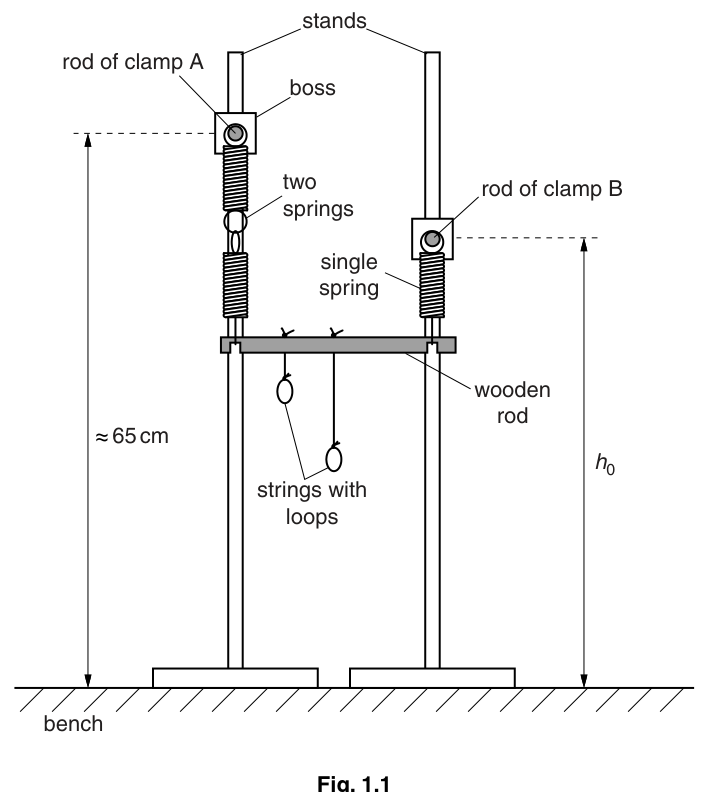
Place the rod of clamp A, supporting the two springs, approximately $65\ \text{cm}$ above the bench.

Once fixed do not change the position of the rod of clamp A throughout the experiment.

Suspend the wooden rod, with strings attached, using the springs as shown. Adjust the position of the rod of clamp B until the wooden rod is horizontal.

Ensure the springs hang vertically.

DifficultyMedium-Easy

Worked solution

Answer

Fix clamp A so that its rod (supporting the two springs) is about $65\ \text{cm}$ above the bench and do not move it.
Suspend the wooden rod using the springs.
Adjust clamp B until the wooden rod is horizontal.
Check the springs hang vertically.

Final answer

Apparatus set up with clamp A fixed, clamp B adjusted so rod is horizontal, springs vertical.

Detailed explanation

Background Concept

In spring experiments, the measured extension must correspond to a change in spring length caused only by the load. If the springs are not vertical, the tension in each spring has a horizontal component and the vertical component is no longer equal to the weight being supported. This changes the effective extension and increases uncertainty.

Understanding the Question

You are being told to build the apparatus exactly as shown and to keep clamp A fixed. Clamp B is then adjusted so the wooden rod is horizontal, both initially and after adding masses. The distance $h$ (and initially $h_0$ ) is measured from the centre of the clamp B rod down to the bench.

Approach

Set a fixed reference by clamping A at a constant height.
Use clamp B to level the wooden rod (so the geometry is consistent for each reading).
Make sure springs hang vertically so the forces are vertical and the extension is reliable.

Step-by-Step Reasoning

Fixing clamp A means the left-hand support height does not change; this reduces an extra variable.
Adjusting clamp B until the wooden rod is horizontal ensures that the measured change in $h$ is linked consistently to the extensions of the spring arrangement.
Vertical springs ensure the extension corresponds to vertical loading only.

Key Takeaways

Keep one part fixed to control variables.
Leveling/aligning reduces systematic error.
Vertical alignment of springs is essential for valid force-extension behaviour.

Common Mistakes

Moving clamp A after the start (changes the reference and ruins comparisons).
Leaving springs angled (introduces horizontal force components).
Judging “horizontal” by eye without careful adjustment.

Things to Be Careful About

Ensure the wooden rod is truly horizontal each time before measuring.
Springs should not rub against stands/strings.
Avoid oscillations before taking readings (wait for the rod to come to rest).

Techniques used

assemble the apparatus as shown in the diagramadjust a clamp height to level a beamensure springs hang vertically to avoid sideways components

(ii)

Measure and record the distance $h_0$ between the centre of the rod of clamp B (supporting the single spring) and the bench.

$h_0$ = ______ $\text{m}$

DifficultyEasy

Worked solution

Answer

Measure $h_0$ from the bench to the centre of the rod of clamp B.

Example (to nearest $1\ \text{mm}$ ):

h_0 = 0.650\ \text{m}

Final answer

0.650 m (example)

Detailed explanation

Background Concept

A height measurement like $h_0$ is a direct length measurement. Good practice is to:

use a clear reference point (here, the centre of the rod of clamp B),
keep the rule vertical,
avoid parallax by reading at eye level.

Understanding the Question

You must measure the initial distance $h_0$ between the bench and the centre of the clamp B rod (the rod that supports the single spring). This is your baseline reading before additional masses are added.

Approach

Place a metre rule with its zero at the bench.
Sight horizontally to the centre of the clamp B rod.
Record the reading in metres with appropriate precision (typically $\pm 1\ \text{mm}$ for a metre rule).

Step-by-Step Reasoning

Align the metre rule so it is vertical and its scale is close to the clamp B rod.
Identify the centre of the clamp rod (not the top or bottom edge).
Read the scale at eye level.
Convert to metres if necessary and record.

Key Takeaways

Define exactly what points the distance is between.
Record to the instrument precision.

Common Mistakes

Measuring to the top of the clamp or the spring instead of the centre of the rod.
Parallax error from reading at an angle.
Mixing units (e.g. writing cm when the answer line asks for m).

Things to Be Careful About

Use consistent precision for all height readings ( $h_0$ and $h$ ).
Ensure the bench reference point is the same each time (same surface).

Techniques used

measure a vertical distance using a metre ruleread a scale at eye level to avoid parallaxrecord a value to appropriate precision

(b)

(i)

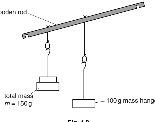
Add masses to the wooden rod as shown in Fig. 1.2. The $100\ \text{g}$ mass hanger should be attached to the longer, central string.

Fig. 1.2

DifficultyEasy

Worked solution

Answer

Attach the $100\ \text{g}$ mass hanger to the longer central string and attach the mass $m$ to the left loop as shown.

Final answer

100 g on central string; mass m on left loop.

Detailed explanation

Background Concept

In practical work, changing where the load is applied changes the torques on the wooden rod and therefore changes how much each spring stretches. For a fair investigation, the arrangement must match the diagram and the central load must be kept constant as instructed.

Understanding the Question

You must add masses exactly as in Fig. 1.2:

a fixed $100\ \text{g}$ mass hanger on the central longer string,
a variable mass $m$ on the left side.

Approach

Place the correct mass on the correct string.
Make sure masses hang freely and do not touch the bench or stands.

Step-by-Step Reasoning

The $100\ \text{g}$ hanger is a control load: it must not change during the rest of the experiment.
The variable $m$ is the independent variable: you will change it to see how the extension changes.

Key Takeaways

Correct placement of masses is essential for valid and repeatable readings.

Common Mistakes

Swapping the masses (putting $m$ on the central string).
Letting masses rest against the stand/bench (reduces the effective load).

Things to Be Careful About

Ensure the strings are not twisted and the rod can settle.
Add masses gently to avoid large oscillations.

Techniques used

attach masses at the specified positionsensure the stated mass remains constantconfirm the load is applied vertically

(ii)

Adjust the height of the rod of clamp B until the wooden rod is horizontal.

DifficultyEasy

Worked solution

Answer

Adjust the height of clamp B until the wooden rod is horizontal (then allow oscillations to die away).

Final answer

Clamp B adjusted so rod is horizontal.

Detailed explanation

Background Concept

A consistent geometry is needed so that changes in the measured height $h$ reflect changes due to the applied load, not changes due to a tilted rod.

Understanding the Question

After adding the masses, the rod will generally tilt. You must move clamp B up or down until the rod is horizontal again, and only then measure $h$ .

Approach

Adjust clamp B slowly.
Check that the rod is level (horizontal) before reading.

Step-by-Step Reasoning

Adding load changes extensions; the right side must be adjusted to restore the horizontal condition.
Once horizontal, the reading of $h$ corresponds to a consistent configuration for comparison across different values of $m$ .

Key Takeaways

Always return the apparatus to the same reference condition before measuring.

Common Mistakes

Measuring $h$ while the rod is still tilted.
Taking readings while the rod is oscillating.

Things to Be Careful About

Tighten clamps after adjustment so they do not slip.
Judge horizontal carefully (small tilt causes systematic changes in $h$ ).

Techniques used

adjust clamp position to level a beamcheck alignment before taking readings

(iii)

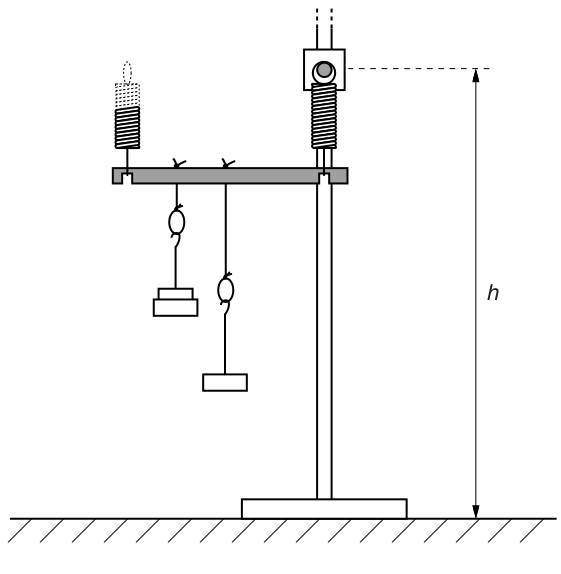
Measure and record the distance $h$ between the centre of the rod of clamp B and the bench, as shown in Fig. 1.3.

Fig. 1.3

$h$ = ______

DifficultyEasy

Worked solution

Answer

Measure $h$ from the bench to the centre of the rod of clamp B.

Example (to nearest $1\ \text{mm}$ ):

h = 0.630\ \text{m}

Final answer

0.630 m (example)

Detailed explanation

Background Concept

To observe the extension caused by added load, you measure the change in height at a defined reference point. Consistency (same points, same instrument, same precision) is crucial.

Understanding the Question

With the rod horizontal (after adjustment), you measure the distance $h$ from the bench to the centre of the clamp B rod.

Approach

Use the same technique as for $h_0$ .
Ensure the rod is horizontal and stationary.

Step-by-Step Reasoning

Wait for oscillations to stop.
Place/hold the metre rule vertically from bench to the level of the clamp B rod.
Read at eye level and record in metres.

Key Takeaways

$h$ is the measurement that changes when the load $m$ changes.

Common Mistakes

Measuring from a different point than used for $h_0$ .
Recording $h$ in cm when other calculations use m.

Things to Be Careful About

Keep the same datum (bench surface) each time.
Avoid parallax and keep the rule vertical.

Techniques used

measure a vertical distance using a metre rulerecord the reading to consistent precisionensure the system is at rest before measuring

(iv)

Calculate the value of $(h_0 - h)$ .

$(h_0 - h)$ = ______

DifficultyEasy

Worked solution

Working

(h_0-h) = 0.650 - 0.630 = 0.020\ \text{m}

Answer

(h_0-h) = 0.020\ \text{m}

Final answer

0.020 m (example)

Detailed explanation

Background Concept

The change $(h_0-h)$ represents how much the clamp B height had to be reduced (or increased) to restore the rod to horizontal after adding load. It is treated as the extension-related change for analysis.

Understanding the Question

You have measured $h_0$ (initial) and $h$ (with mass $m$ ). You must calculate the difference $h_0-h$ .

Approach

Ensure both $h_0$ and $h$ are in the same unit (metres).
Subtract in the correct order: initial minus new.

Step-by-Step Reasoning

Because the added mass makes the system extend more, typically $h$ is smaller than $h_0$ , so $h_0-h$ is positive.
Do the subtraction and keep the result to a consistent decimal place based on the measurement precision.

Key Takeaways

Derived values must keep consistent units and sensible precision.

Common Mistakes

Reversing the subtraction and getting a negative value.
Mixing cm and m.

Things to Be Careful About

If $h$ happens to be slightly larger than $h_0$ due to adjustment/reading error, re-check leveling and readings before proceeding.

Techniques used

calculate a difference between two measured valuesuse consistent units and precision in derived quantities

(c)

By increasing the mass $m$ , repeat (b)(ii), (b)(iii) and (b)(iv) until you have five sets of values of $m$ and $h$ . Do not change the mass attached to the longer, central string.

Include values of $\frac{(h_0 - h)}{m}$ and $\frac{1}{m}$ in your table.

10M

DifficultyMedium

Worked solution

Answer

Obtain at least five sets of readings of $m$ and $h$ (keeping the central $100\ \text{g}$ mass hanger constant) and calculate $(h_0-h)$ , $\dfrac{(h_0-h)}{m}$ and $\dfrac{1}{m}$ .

Example of a suitable table (using $h_0 = 0.650\ \text{m}$ ):

$m\ /\ \text{kg}$	$h\ /\ \text{m}$	$(h_0-h)\ /\ \text{m}$	$\dfrac{(h_0-h)}{m}\ /\ \text{m kg}^{-1}$	$\dfrac{1}{m}\ /\ \text{kg}^{-1}$
0.150	0.630	0.020	0.133	6.67
0.200	0.625	0.025	0.125	5.00
0.250	0.620	0.030	0.120	4.00
0.300	0.615	0.035	0.117	3.33
0.350	0.610	0.040	0.114	2.86

Final answer

See table (student-dependent).

Detailed explanation

Background Concept

Good practical data must be sufficient in quantity and range to reveal a trend and support later graphing. A results table should:

include all raw readings (here $m$ and $h$ ),
include all derived quantities required by the question,
have clear headings with quantity and unit,
use consistent precision within each column.

Understanding the Question

You are told to repeat the procedure for increasing mass $m$ until you have five sets of values of $m$ and $h$ . You must not change the mass on the central long string (a control). Your table must also include two calculated columns:

\frac{(h_0-h)}{m}, \quad \frac{1}{m}

Approach

Choose at least five different values of $m$ with a sensible spread.
For each $m$ : level the rod, measure $h$ , compute $(h_0-h)$ .
Calculate the two required derived quantities and record all values in one table.

Step-by-Step Reasoning

Independent variable: $m$ (you choose the values).
Dependent reading: $h$ (measured after leveling each time).
Derived extension-type value: $(h_0-h)$ .
Derived graph variables:
- $y = \dfrac{(h_0-h)}{m}$ (units $\text{m kg}^{-1}$ )
- $x = \dfrac{1}{m}$ (units $\text{kg}^{-1}$ )

Precision guidance:

If $h$ is measured to the nearest $1\ \text{mm}$ , record $h$ and $h_0$ to $0.001\ \text{m}$ .
Then $(h_0-h)$ should also be to $0.001\ \text{m}$ .
For calculated columns, a typical convention is 3 s.f. (or consistent decimal places) across the column.

Repeat readings:

If time allows, repeating $h$ for the same $m$ and averaging can improve reliability; at minimum, ensure readings are steady and repeatable.

Key Takeaways

A high-scoring table has correct headings, units, consistent precision, and enough data points.
Control variables (here the central $100\ \text{g}$ hanger) must be kept constant.

Common Mistakes

Missing units in column headings.
Only giving $m$ and $h$ but not the required calculated columns.
Using grams in some places and kilograms in others (causes wrong $1/m$ and wrong graph scale).
Inconsistent decimal places within a column.

Things to Be Careful About

Do not change the central mass hanger at any stage.
Ensure the rod is horizontal before every $h$ reading.
Avoid too narrow a range of $m$ (it makes the graph less reliable and gradients more uncertain).

Techniques used

take multiple readings over a suitable range of the independent variablecalculate derived quantities for each runrecord data in a single table with correct headings and unitskeep a control variable constant throughout

(d)

(i)

Plot a graph of $\frac{(h_0 - h)}{m}$ on the $y$ -axis against $\frac{1}{m}$ on the $x$ -axis.

DifficultyMedium

Worked solution

Answer

Plot a graph with:

$x$ -axis: $\dfrac{1}{m}\ /\ \text{kg}^{-1}$
$y$ -axis: $\dfrac{(h_0-h)}{m}\ /\ \text{m kg}^{-1}$

Use a suitable scale (at least half the grid) and plot all five points from the table.

Final answer

Graph plotted (student-dependent).

Detailed explanation

Background Concept

A graph is used to identify linear relationships and to allow gradient/intercept measurements. Marks are typically awarded for:

correct axis choice,
correct labels and units,
sensible scales,
accurate points.

Understanding the Question

You must plot the transformed variables

y = \frac{(h_0-h)}{m} \quad \text{against} \quad x = \frac{1}{m}

with $y$ on the vertical axis and $x$ on the horizontal axis.

Approach

Decide the range of your $x$ and $y$ values from your table.
Choose scales that are easy to use (e.g. 1 large square = 0.5 or 1.0 in the chosen units), and that spread the points across most of the graph.
Label each axis with both the expression and the unit.

Step-by-Step Reasoning

From your table, locate each point $(1/m,\ (h_0-h)/m)$ .
Plot with small, neat crosses.
Check a couple of points by re-reading from your table to avoid transcription errors.

Key Takeaways

The axis variables must match the question exactly.
Units in labels prevent losing marks.

Common Mistakes

Swapping axes (plotting $y$ against $x$ the wrong way round).
Forgetting units or writing incorrect units (e.g. using g instead of kg).
Using a cramped scale so points occupy a small corner of the grid.

Things to Be Careful About

Use the same value of $m$ (in kg) for both $1/m$ and $(h_0-h)/m$ .
Ensure the plotted point positions reflect the correct number of decimal places (do not round too aggressively before plotting).

Techniques used

choose suitable axis scales that use most of the gridlabel axes with quantity and unitplot data points accurately

(ii)

Draw the straight line of best fit.

DifficultyMedium-Easy

Worked solution

Answer

Draw a single straight line of best fit through the plotted points (balanced so there are roughly equal deviations above and below the line).

Final answer

Best-fit straight line drawn (student-dependent).

Detailed explanation

Background Concept

A best-fit line represents the overall trend of data with random scatter. In Cambridge practical marking, a best-fit line should be:

a single straight line (not point-to-point),
drawn with a ruler,
positioned to balance the scatter.

Understanding the Question

After plotting the points from (d)(i), you must draw the straight line that best represents the relationship.

Approach

Use a ruler.
Visually balance the line so the deviations are similar above and below.
Do not force the line through the origin unless the points and relationship clearly justify it.

Step-by-Step Reasoning

Identify the general linear trend.
Place the ruler so that the line passes centrally through the cluster.
Draw a long line across most of the graph area to help with accurate gradient determination.

Key Takeaways

A best-fit line is about the overall trend, not connecting points.

Common Mistakes

Joining the dots.
Drawing a line that passes through every point even when scatter exists.
Drawing a very short line segment (reduces gradient accuracy).

Things to Be Careful About

If one point is a clear anomaly, do not automatically force the line through it; check the corresponding table entry for mistakes first.

Techniques used

draw a single straight line of best fit balancing scatterignore minor random scatter rather than joining points

(iii)

Determine the gradient and $y$ -intercept of this line.

gradient = ______
$y$ -intercept = ______

DifficultyMedium

Worked solution

Working

Using two well-separated points on the best-fit line (example):

(x_1,y_1)=(2.86,0.114),\quad (x_2,y_2)=(6.67,0.133)

\text{gradient} = \frac{\Delta y}{\Delta x} = \frac{0.133-0.114}{6.67-2.86} = \frac{0.019}{3.81}=4.99\times 10^{-3}\ \text{m}

$y$ -intercept (from best-fit line, example):

y\text{-intercept}=0.100\ \text{m kg}^{-1}

Answer

gradient $= 5.0\times 10^{-3}\ \text{m}$

$y$ -intercept $= 0.100\ \text{m kg}^{-1}$

Final answer

gradient = 5.0×10^-3 m, y-intercept = 0.100 m kg^-1 (example)

Detailed explanation

Background Concept

For a straight-line graph of the form

y = mx + c

the gradient is $m = \Delta y / \Delta x$ ,
the y-intercept is $c$ (the value of $y$ when $x=0$ ).

The units come directly from the axis units:

here $y$ has units $\text{m kg}^{-1}$ ,
here $x$ has units $\text{kg}^{-1}$ ,
so the gradient has units

\frac{\text{m kg}^{-1}}{\text{kg}^{-1}} = \text{m}.

Understanding the Question

You must read the gradient and y-intercept of your best-fit line on the graph of $\dfrac{(h_0-h)}{m}$ against $\dfrac{1}{m}$ .

Approach

Use a large triangle on the best-fit line: pick two points far apart on the line (not necessarily your plotted data points).
Compute $\Delta y$ and $\Delta x$ from the graph readings.
Find the y-intercept by extending the line to $x=0$ and reading $y$ .

Step-by-Step Reasoning

diagram-graph

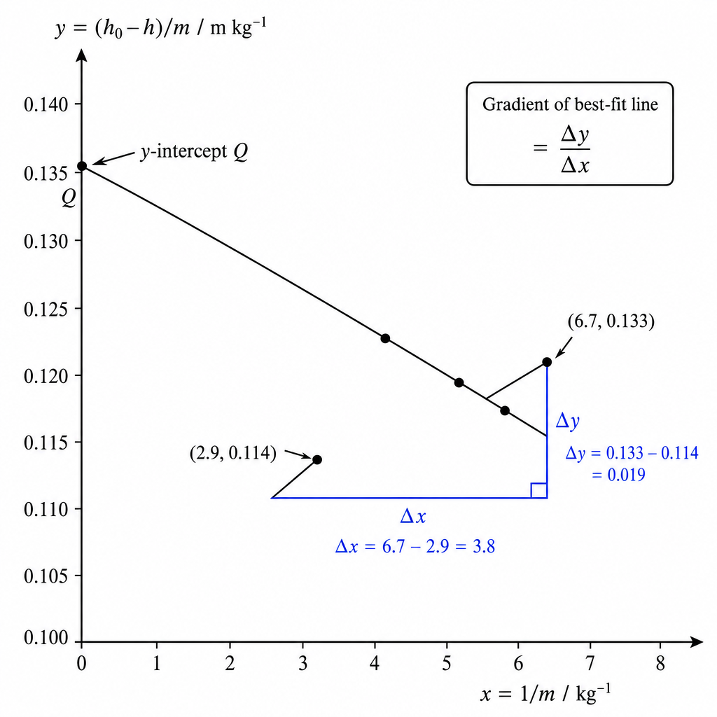
Choose two points on the drawn line that are widely separated to reduce percentage reading error.
Read off $x_1, y_1$ and $x_2, y_2$ .
Calculate

\text{gradient} = \frac{y_2-y_1}{x_2-x_1}.

Then extend the line back to where it crosses the y-axis ( $x=0$ ) and read the intercept.

If your line is slightly scattered, different sensible choices of points may give slightly different gradients; your best-fit line choice is meant to minimise this.

Key Takeaways

Gradient: always $\Delta y/\Delta x$ using the best-fit line.
Intercept: read at $x=0$ .
Units: taken from axis labels.

Common Mistakes

Using $\Delta x/\Delta y$ instead of $\Delta y/\Delta x$ .
Using two plotted points that are close together (gives a large gradient uncertainty).
Forgetting to include units, or giving gradient the wrong units.

Things to Be Careful About

Use the best-fit line, not a point-to-point join.
Read coordinates carefully; use the full graph scale, not rounded-off values.
The intercept is at $x=0$ even if your smallest $x$ value is not near zero (you may need to extend the line).

Techniques used

determine gradient using a large triangle on the best-fit lineread y-intercept from the best-fit lineuse correct units from axis labels

(e)

The quantities $h$ and $m$ are related by the equation

\frac{(h_0 - h)}{m} = \frac{P}{m} + Q

where $P$ and $Q$ are constants.

Use your answers in (d)(iii) to determine the values of $P$ and $Q$ . Give appropriate units.

$P$ = ______
$Q$ = ______

DifficultyMedium-Easy

Worked solution

Working

Given

\frac{(h_0-h)}{m} = \frac{P}{m} + Q

Let

y = \frac{(h_0-h)}{m},\quad x = \frac{1}{m}

Then

y = Px + Q

So gradient $=P$ and y-intercept $=Q$ .

Answer

P = 5.0\times 10^{-3}\ \text{m}

Q = 0.100\ \text{m kg}^{-1}

Final answer

P = 5.0×10^-3 m, Q = 0.100 m kg^-1 (example)

Detailed explanation

Background Concept

Many practicals convert a relationship into straight-line form:

y = mx + c.

If you plot $y$ against $x$ , then:

gradient $m$ is the coefficient of $x$ ,
intercept $c$ is the constant term.

Units:

$y = (h_0-h)/m$ has units $\text{m kg}^{-1}$ ,
$x = 1/m$ has units $\text{kg}^{-1}$ ,
so the gradient has units $\text{m}$ and the intercept has units $\text{m kg}^{-1}$ .

Understanding the Question

You are given

\frac{(h_0-h)}{m} = \frac{P}{m} + Q

and you have already plotted $\dfrac{(h_0-h)}{m}$ (y-axis) against $\dfrac{1}{m}$ (x-axis) and found the gradient and intercept. You must now state the values of $P$ and $Q$ with correct units.

Approach

Rewrite the equation in terms of your plotted variables.
Compare directly to $y = mx + c$ .
Read off $P$ and $Q$ from gradient and intercept.

Step-by-Step Reasoning

Define

y = \frac{(h_0-h)}{m},\quad x = \frac{1}{m}.

Then

\frac{P}{m} = P\left(\frac{1}{m}\right)=Px,

so the given equation becomes

y = Px + Q.

Therefore:

$P$ is the gradient of the graph,
$Q$ is the y-intercept.

Units follow from dimensional comparison:

Since $y$ is $\text{m kg}^{-1}$ and $x$ is $\text{kg}^{-1}$ , the coefficient $P$ must be in metres.
$Q$ must have the same units as $y$ , i.e. $\text{m kg}^{-1}$ .

Key Takeaways

Always match your graph variables to the algebraic straight-line form.
Constants are identified by comparing with $y = mx + c$ .
Units can be checked from axis units.

Common Mistakes

Swapping $P$ and $Q$ .
Giving incorrect units (e.g. $P$ in $\text{m kg}^{-1}$ ).
Using values from a single data point instead of the best-fit gradient/intercept.

Things to Be Careful About

Use the gradient and intercept from the best-fit line (not from raw data points).
Quote values to sensible significant figures consistent with your graph-reading precision.

Techniques used

match an experimental straight-line graph to y = mx + cidentify constants from gradient and interceptdeduce units of constants from the equation

The rest of this paper

1 more questions

Q2Manipulation, Measurement and Observation · Analysis, Conclusions and Evaluation · Presentation of Data and Observations20M

Loading the full paper…