You may not need to use all of the materials provided. In this experiment, you will investigate the equilibrium of a mass and pulley system. (a) The apparatus has been set up in an arrangement similar to that shown in Fig. 1.1. (b) Measure and record the height $H$ of the central knot above the bench. $H$ = \_\_\_\_\_\_ $\text{m}$ (i) Suspend the mass hanger from the central loop as shown in Fig. 1.2. (ii) Record the central suspended mass $m$. $m$ = \_\_\_\_\_\_ $\text{kg}$…

(a) Apparatus identified; H is the vertical height of the central knot above the bench. · (b) Example: H = 0.650 m · (c)(i) Central mass hanger attached and allowed to reach equilibrium. · (c)(ii) Example: m = 0.100 kg · (c)(iii) Example: h = 0.580 m · (c)(iv) Example: y = 0.070 m · (d) Six-row results table including m, h, y, 1/y^2 and 1/m^2 with correct headings/units (values student-dependent). · (e)(i) Graph of 1/y^2 (y-axis) against 1/m^2 (x-axis), correctly labelled…

Physics 9702/36 — October/November 2011

Cambridge AS Level · Advanced Practical Skills · worked solutions for every part, with the mark scheme

questions

marks

120

minutes

Topics Manipulation, Measurement and Observation · Presentation of Data and Observations · Analysis, Conclusions and Evaluation

Q1Manipulation, Measurement and ObservationPresentation of Data and ObservationsAnalysis, Conclusions and EvaluationFree sample

You may not need to use all of the materials provided.

In this experiment, you will investigate the equilibrium of a mass and pulley system.

(a)

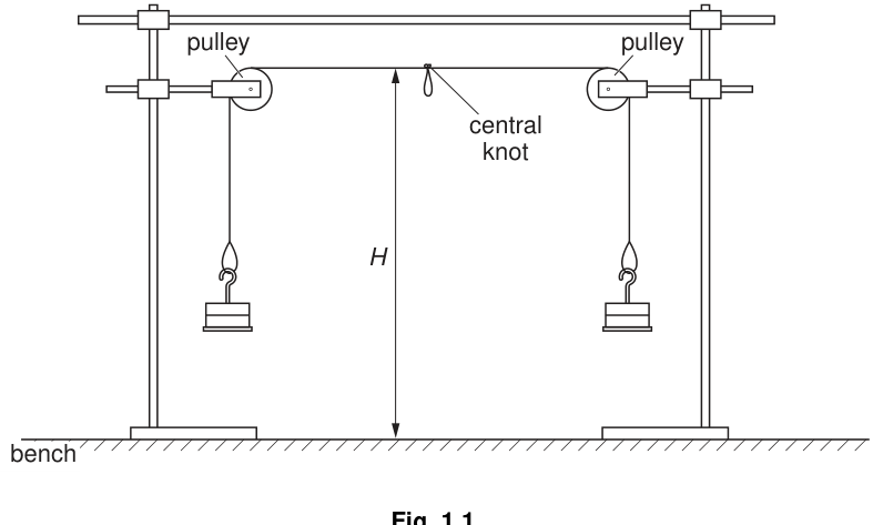
The apparatus has been set up in an arrangement similar to that shown in Fig. 1.1.

Fig. 1.1

DifficultyEasy

Worked solution

Answer

Apparatus as shown: string over two pulleys with two end hangers; central knot between pulleys. Height $H$ is measured vertically from the bench to the central knot (with the system at rest).

Final answer

Apparatus identified; H is the vertical height of the central knot above the bench.

Detailed explanation

Background Concept

In practical mechanics, a diagram is used to define what is being measured and the reference level for measurements. A “height above the bench” is a vertical distance measured from the bench surface (reference level) to the point of interest.

In pulley-string systems, you must also ensure the system is stationary before taking readings so the geometry (and hence the measured heights) is well-defined.

Understanding the Question

You are told the apparatus is already set up similar to Fig. 1.1. The key point is to recognise:

two pulleys fixed to a horizontal bar,
a single string passing over both pulleys,
mass hangers at the two ends,
a central knot/loop in the middle of the string.

The quantity $H$ is defined as the vertical distance from the bench surface up to the central knot.

Approach

Use the diagram to:

identify the correct point to measure to (the central knot),
identify the correct reference level (the bench surface),
ensure the system is at rest so the knot position is stable.

Step-by-Step Reasoning

Locate the central knot between the pulleys.
Visualise a vertical line from the bench surface up to the knot: that is $H$ .
Ensure the string and hangers are not swinging; wait for equilibrium.

Key Takeaways

Always state the reference level for heights.
Ensure equilibrium (no motion) before measuring a position.

Common Mistakes

Measuring to the pulley axle or to the horizontal bar instead of the knot.
Measuring along the string (a slanted distance) instead of vertically.
Taking readings while the knot is still oscillating.

Things to Be Careful About

Parallax: your eye should be level with the knot when reading a rule.
The bench surface must be the same reference level used throughout the experiment.

Techniques used

identify the measured quantities from the apparatus diagramcheck the reference level used for a height measurementensure the system is stationary before taking readings

(b)

Measure and record the height $H$ of the central knot above the bench.

$H$ = ______ $\text{m}$

DifficultyEasy

Worked solution

Answer

Measure $H$ with a metre rule held vertically (eye level with the knot).

Example:

H = 0.650\ \text{m}

Final answer

Example: H = 0.650 m

Detailed explanation

Background Concept

A height measurement is a vertical displacement between two levels. A metre rule typically has 1 mm smallest divisions, so a sensible recording precision is to the nearest 1 mm, i.e. $\pm 0.5\ \text{mm}$ uncertainty, and record $H$ to $0.001\ \text{m}$ .

Understanding the Question

You must measure the height $H$ of the central knot above the bench in the initial arrangement (before the central mass is added). The answer space shows the unit is metres, so you should record in $\text{m}$ .

Approach

Place/hold the rule vertically with its zero at the bench surface.
Read the value at the central knot.
Record $H$ in metres to an appropriate number of decimal places.

Step-by-Step Reasoning

Align the metre rule so it is vertical and close to the knot.
Make sure the zero of the rule corresponds to the bench surface (not the clamp base or some other point).
Bring your eye level with the knot to avoid parallax.
Read and record $H$ with consistent precision (e.g. $0.650\ \text{m}$ ).

Key Takeaways

Measure vertically from the stated reference level.
Record to the resolution of the measuring instrument.

Common Mistakes

Writing the unit as cm even though the answer line specifies metres.
Recording too few decimal places (e.g. $0.65\ \text{m}$ ) when a mm-scale rule was used.
Measuring from the floor instead of the bench.

Things to Be Careful About

If the knot is thick, decide a consistent point (e.g. the centre of the knot) and use it every time.
Ensure the system is stationary when reading.

Techniques used

measure a vertical height using a metre ruleavoid parallax when reading a scalerecord a reading to the appropriate precision

(c)

(i)

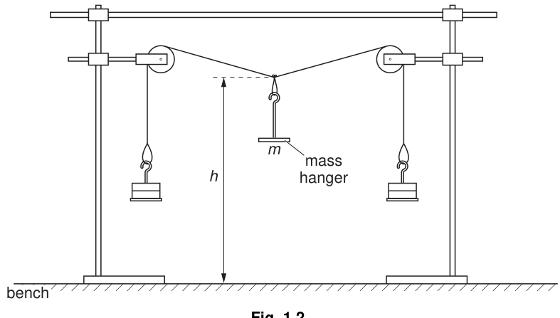
Suspend the mass hanger from the central loop as shown in Fig. 1.2.

Fig. 1.2

DifficultyEasy

Worked solution

Answer

Suspend the mass hanger from the central loop/knot so it hangs freely and allow the system to come to rest before taking readings of $m$ and $h$ .

Final answer

Central mass hanger attached and allowed to reach equilibrium.

Detailed explanation

Background Concept

In equilibrium experiments, the key requirement is a stable, repeatable geometry. Adding a load at the central knot changes the shape of the string and lowers the knot to a new position (height $h$ ). Measurements are only meaningful once the system is stationary.

Understanding the Question

You must attach a third hanger of mass $m$ at the central knot/loop as in Fig. 1.2. This creates a new height $h$ for the knot.

Approach

Attach the hanger securely at the central loop.
Ensure it does not touch the bench or other parts of the apparatus.
Wait for oscillations to stop.

Step-by-Step Reasoning

Hook the central hanger onto the loop at the knot.
Check the string sits correctly in the pulley grooves.
If the knot swings, wait until it becomes still; only then measure $h$ .

Key Takeaways

Equilibrium readings require the system to be at rest.
The hanger must hang freely for the force to be vertical.

Common Mistakes

Taking $h$ while the knot is still moving.
The central hanger rubbing against a stand, changing the effective forces.

Things to Be Careful About

Make sure the knot/loop does not slip along the string when the mass is added.
Ensure both end masses remain suspended and the string stays taut.

Techniques used

attach a mass hanger securely to a loop/knotcheck that the hanger hangs freely without obstructionallow oscillations to die away before proceeding

(ii)

Record the central suspended mass $m$ .

$m$ = ______ $\text{kg}$

DifficultyEasy

Worked solution

Answer

Record the total central suspended mass (hanger + any added masses) in $\text{kg}$ .

Example:

m = 0.100\ \text{kg}

Final answer

Example: m = 0.100 kg

Detailed explanation

Background Concept

Masses in practical work are usually supplied as slotted masses labelled in grams. The exam requires SI units, so you should convert to kilograms:

1\ \text{g} = 1.0\times 10^{-3}\ \text{kg}

The total suspended mass is the mass of the hanger plus all masses added to it.

Understanding the Question

You must write down the value of $m$ for the mass hanging from the central loop. This $m$ is then varied later, so it must be recorded accurately.

Approach

Add up all components of the central load.
Convert to $\text{kg}$ .
Record with sensible precision (typically to $0.001\ \text{kg}$ if masses are in $1\ \text{g}$ steps).

Step-by-Step Reasoning

If the hanger is, for example, $50\ \text{g}$ and you add $50\ \text{g}$ , the total is $100\ \text{g}$ .
Convert: $100\ \text{g} = 0.100\ \text{kg}$ .
Record $m$ clearly with unit.

Key Takeaways

Always use the total suspended mass.
Convert g to kg correctly.

Common Mistakes

Recording only the added masses and forgetting the hanger mass.
Leaving the answer in grams.

Things to Be Careful About

Keep consistent increments in $m$ so you get a good spread of data later.
Ensure the labelled masses are secure so they do not fall during measurements.

Techniques used

determine the total suspended mass by summing hanger and added massesconvert grams to kilograms correctlyrecord the mass to an appropriate precision

(iii)

Measure and record the height $h$ of the central knot above the bench, as shown in Fig. 1.2.

$h$ = ______ $\text{m}$

DifficultyEasy

Worked solution

Answer

With the central mass attached and the system at rest, measure $h$ vertically from the bench to the central knot.

Example:

h = 0.580\ \text{m}

Final answer

Example: h = 0.580 m

Detailed explanation

Background Concept

When a load changes, the system moves to a new equilibrium. The measured quantity $h$ is a vertical height, so it must be taken in the same way as $H$ to make the subtraction $H-h$ meaningful.

Random uncertainty can be reduced by taking repeat readings and averaging.

Understanding the Question

After attaching the central mass, the knot moves down. You must measure and record the new height $h$ above the bench.

Approach

Wait until motion stops.
Measure vertically from the same reference level (bench) to the same point (knot).
Record $h$ to the same precision as $H$ .

Step-by-Step Reasoning

Ensure the central hanger is not swinging.
Place the rule vertically close to the knot.
Read $h$ at eye level.
If time allows, read $h$ twice and take the mean.

Key Takeaways

Consistency between $H$ and $h$ measurements is crucial.
Repeat readings help reliability.

Common Mistakes

Measuring to a different point on the knot than was used for $H$ .
Recording $h$ to a different precision than $H$ .

Things to Be Careful About

If the bench is not level or the rule cannot touch the bench directly, use a fixed reference (e.g. a block of known height) consistently for both $H$ and $h$ and correct appropriately.

Techniques used

measure a new equilibrium height after changing a loadreduce random error by repeating a reading and averagingrecord consistent decimal places

(iv)

Calculate the deflection $y$ , where $y = (H - h)$ .

$y$ = ______ $\text{m}$

DifficultyEasy

Worked solution

Working

y = (H-h)

Example:

y = 0.650 - 0.580 = 0.070\ \text{m}

Answer

y = 0.070\ \text{m}

Final answer

Example: y = 0.070 m

Detailed explanation

Background Concept

A deflection is a change in position. Here the deflection $y$ is defined explicitly as:

y = H - h

So $y$ is positive because adding the central mass makes the knot move down, meaning $h$ is smaller than $H$ .

For subtraction, the decimal places in the result should match the least precise of the two readings.

Understanding the Question

You are given $H$ (initial height) and have measured $h$ (new height). You must calculate the deflection $y$ and record it in metres.

Approach

Substitute your measured values into $y = H - h$ .
Keep units consistent (both in metres).
Record $y$ to an appropriate precision.

Step-by-Step Reasoning

Using the example values:

$H = 0.650\ \text{m}$ , $h = 0.580\ \text{m}$ .
Subtract:

y = 0.650 - 0.580 = 0.070\ \text{m}

The unit stays as metres because it is a difference of two lengths.

Key Takeaways

Derived quantities must be calculated using the defined formula.
Units and precision must be consistent with the measurements.

Common Mistakes

Doing $h-H$ and getting a negative deflection.
Mixing units (e.g. $H$ in cm and $h$ in m).

Things to Be Careful About

If your values of $H$ and $h$ are close, $y$ may be small; keep enough decimal places so $y$ is not rounded to zero.

Techniques used

calculate a derived quantity from two measured valuespropagate consistent decimal places in subtractionstate the result with the correct unit

(d)

Change $m$ by adding masses to the hanger suspended from the central loop and repeat (c)(ii), (c)(iii) and (c)(iv) until you have six sets of values for $m$ , $h$ and $y$ .

Include in your table of results values for $\frac{1}{y^2}$ and $\frac{1}{m^2}$ .

10M

DifficultyMedium-Hard

Worked solution

Answer

Obtain six different values of $m$ (using a wide range). For each $m$ measure $h$ , calculate $y = H-h$ , then calculate and record $1/y^2$ and $1/m^2$ .

Record all values in one table with headings (quantity and unit), e.g.

$m / \text{kg}$
$h / \text{m}$
$y / \text{m}$
$1/y^2 / \text{m}^{-2}$
$1/m^2 / \text{kg}^{-2}$

Example calculation (for one row):

\frac{1}{y^2} = \frac{1}{(0.070)^2} = 204\ \text{m}^{-2}

\frac{1}{m^2} = \frac{1}{(0.100)^2} = 100\ \text{kg}^{-2}

Final answer

Six-row results table including m, h, y, 1/y^2 and 1/m^2 with correct headings/units (values student-dependent).

Detailed explanation

Background Concept

Good experimental data must be:

sufficient in quantity (enough data points to identify a trend),
wide in range (so the graph has a reliable gradient),
recorded clearly (single table, correct headings, units),
processed correctly (derived quantities calculated for every row).

Here, the experiment ultimately needs a straight-line plot of $1/y^2$ against $1/m^2$ , so you must compute these two derived columns.

Understanding the Question

You must vary the central mass $m$ and repeat measurements until you have six sets of $m$ , $h$ and $y$ . You must also include $1/y^2$ and $1/m^2$ in the same table.

Approach

Choose six values of $m$ spanning a good range (e.g. equal steps).
For each $m$ :

wait for equilibrium,
measure $h$ ,
compute $y = H-h$ ,
compute $1/y^2$ and $1/m^2$ .

Tabulate everything with correct units and consistent precision.

Step-by-Step Reasoning

Choosing the range: If all $m$ values are too similar, $1/m^2$ changes little, making the gradient uncertain. Use the full set of masses to spread $m$ .
Measuring $h$ reliably: take repeat readings of $h$ if possible and average to reduce random error.
Calculating $y$ :

y = H - h

Calculating the derived columns:

\frac{1}{y^2} = y^{-2}, \qquad \frac{1}{m^2} = m^{-2}

Use your calculator carefully with brackets.

Table conventions: headings should be in the form “quantity / unit” and all entries in a column should have consistent decimal places where appropriate.

Key Takeaways

Six well-spaced data points improve the reliability of a straight-line graph.
A clear table with correct units and consistent precision is essential.
Derived quantities must be calculated for every row.

Common Mistakes

Only taking a narrow range of $m$ values.
Forgetting to include $1/y^2$ and $1/m^2$ columns.
Writing headings without units, or writing units in the data cells inconsistently.
Calculator error: using $1/y^2$ as $(1/y)^2$ is fine mathematically, but missing brackets can cause mistakes.

Things to Be Careful About

If $y$ is small, $1/y^2$ becomes very large; keep enough significant figures in $y$ so rounding does not dominate.
Ensure $m$ is in $\text{kg}$ before calculating $1/m^2$ , otherwise your x-axis values (and gradient units) will be wrong.
Keep $H$ the same throughout; if the apparatus shifts, re-measure $H$ and restart so the dataset is consistent.

Techniques used

collect a suitable range of values for the independent variablecalculate derived quantities for each row of dataconstruct a results table with correct headings and unitskeep consistent significant figures within columns

(e)

(i)

Plot a graph of $\frac{1}{y^2}$ on the $y$ -axis against $\frac{1}{m^2}$ on the $x$ -axis.

DifficultyMedium

Worked solution

Answer

Plot $1/y^2$ (units $\text{m}^{-2}$ ) on the $y$ -axis against $1/m^2$ (units $\text{kg}^{-2}$ ) on the $x$ -axis.

Use a scale that uses at least half of each axis.
Label each axis with quantity and unit.
Plot all six points accurately.

Final answer

Graph of 1/y^2 (y-axis) against 1/m^2 (x-axis), correctly labelled and scaled (student-dependent).

Detailed explanation

Background Concept

A good graph allows you to determine relationships and constants reliably. Cambridge marking typically rewards:

correct choice of axes,
clear axis labels including units,
sensible scales (not cramped, not awkward),
accurate plotting of points.

Understanding the Question

You have calculated $1/y^2$ and $1/m^2$ for six data sets. You must plot:

vertical axis: $1/y^2$
horizontal axis: $1/m^2$

Approach

Decide suitable axis ranges using your minimum and maximum values.
Choose scales that spread the points over much of the graph paper.
Plot each pair $(1/m^2, 1/y^2)$ as a small, neat cross.

Step-by-Step Reasoning

From your table, identify the smallest and largest $1/m^2$ and $1/y^2$ .
Choose scales (e.g. 1 large square = some convenient value) so points span most of each axis.
Label axes as:

$1/m^2 / \text{kg}^{-2}$ on x-axis
$1/y^2 / \text{m}^{-2}$ on y-axis

Plot all six points accurately.

Key Takeaways

Axis labels must include units.
Good scaling reduces uncertainty in gradient and intercept.

Common Mistakes

Swapping axes (plotting $1/m^2$ on y-axis).
Missing units on axis labels.
Using a scale that compresses points into a small region.

Things to Be Careful About

Do not force the axes to start at zero unless it helps; choose ranges based on your data.
Plotting errors often come from reading the wrong column or misplacing decimal points; double-check each coordinate.

Techniques used

label axes with quantity and unitchoose a sensible scale that uses most of the gridplot points accurately from a results table

(ii)

Draw the straight line of best fit.

DifficultyMedium-Easy

Worked solution

Answer

Draw a single straight line of best fit through the plotted points (not point-to-point), with approximately equal scatter of points above and below the line.

Final answer

Straight line of best fit drawn.

Detailed explanation

Background Concept

A best-fit line represents the overall trend of data with random scatter. For a linear relationship, the best-fit line should:

be straight,
pass through the central trend of the points,
have roughly equal numbers (or equal overall spread) of points on either side.

Understanding the Question

After plotting the points, you must draw the straight line that best represents the relationship between $1/y^2$ and $1/m^2$ .

Approach

Use a ruler.
Do not connect the points one by one.
Ignore small scatter and aim for an overall balance.

Step-by-Step Reasoning

Place the ruler so the line passes through the “middle” of the cluster.
Adjust so the vertical deviations (residuals) look balanced.
Draw the line across most of the graph area to help with intercept readings.

Key Takeaways

The best-fit line is about the trend, not exact passage through every point.

Common Mistakes

Joining successive points instead of drawing a best-fit line.
Forcing the line through the origin when the data do not support it.

Things to Be Careful About

If one point is clearly anomalous, you normally still draw the best-fit line for the main trend; do not “bend” the line to include it.

Techniques used

draw a single straight line that balances the scatter of pointsavoid joining point-to-pointextend the line to read the intercept accurately

(iii)

Determine the gradient and $y$ -intercept of this line.

gradient = ______

$y$ -intercept = ______

DifficultyMedium

Worked solution

Working

Use a large triangle on the best-fit line:

\text{gradient} = \frac{\Delta(1/y^2)}{\Delta(1/m^2)}

Read $y$ -intercept where $1/m^2 = 0$ .

Example (from a typical graph):

\text{gradient} \approx 8.0\times 10^{-3}\ \text{kg}^2\ \text{m}^{-2}

\text{$y$-intercept} \approx -25\ \text{m}^{-2}

Answer

gradient = (from your graph)

$y$ -intercept = (from your graph)

Final answer

Gradient and y-intercept read from the best-fit line (student-dependent).

Detailed explanation

Background Concept

For a straight-line graph, the gradient and intercept come from the general form:

Y = mX + c

where:

$m$ is the gradient (slope),
$c$ is the y-intercept (value of $Y$ when $X=0$ ).

For experimental graphs, gradients should be found using a large triangle on the best-fit line (not between two adjacent data points), because this reduces the percentage uncertainty.

Understanding the Question

Your axes are:

$Y = 1/y^2$ (units $\text{m}^{-2}$ ),
$X = 1/m^2$ (units $\text{kg}^{-2}$ ).

You must determine:

the gradient of the straight best-fit line,
the y-intercept (the value of $1/y^2$ when $1/m^2 = 0$ ).

Approach

Choose two well-separated points on the best-fit line.
Read their coordinates accurately.
Compute:

\text{gradient} = \frac{\Delta Y}{\Delta X}

Read the intercept from where the best-fit line crosses the $Y$ -axis.

Step-by-Step Reasoning

diagram-eiii-1

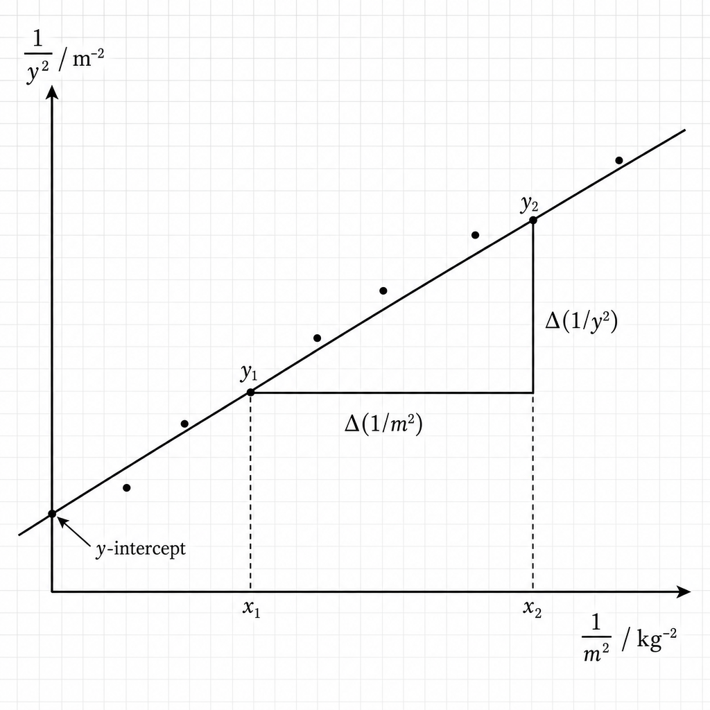
Pick two points far apart on the drawn line (not necessarily actual plotted points), e.g. one near the left and one near the right.
Suppose these points have coordinates $(X_1, Y_1)$ and $(X_2, Y_2)$ .
Compute changes:

\Delta Y = Y_2 - Y_1, \qquad \Delta X = X_2 - X_1

Then:

\text{gradient} = \frac{\Delta Y}{\Delta X}

Units of gradient:

\frac{\text{m}^{-2}}{\text{kg}^{-2}} = \text{kg}^2\ \text{m}^{-2}

The y-intercept is the value of $Y$ at $X=0$ . If the line crosses below zero, the intercept is negative.

Key Takeaways

Use the best-fit line, not point-to-point.
Use a large triangle to reduce uncertainty.
Gradient units come from (y-units)/(x-units).

Common Mistakes

Calculating $\Delta X/\Delta Y$ (inverting the gradient).
Using two nearby points so small reading errors give a large gradient error.
Reading the intercept from a plotted point rather than where the line crosses the axis.

Things to Be Careful About

Always use the same axis variables: here $Y = 1/y^2$ and $X = 1/m^2$ .
Extend the best-fit line far enough to reach the y-axis cleanly so the intercept can be read.
Keep enough significant figures when calculating the gradient so rounding does not dominate.

Techniques used

determine gradient using a large triangle on the best-fit lineread the y-intercept from the graphcalculate a ratio of changes with correct units

(f)

The relationship between $y$ and $m$ is

\frac{1}{y^2} = \frac{p}{m^2} - q

where $p$ and $q$ are constants.

Using your answers from (e)(iii), determine the values of $p$ and $q$ .
Give appropriate units.

$p$ = ______

$q$ = ______

DifficultyMedium-Easy

Worked solution

Working

Given:

\frac{1}{y^2} = \frac{p}{m^2} - q

Let $Y = 1/y^2$ and $X = 1/m^2$ , so:

Y = pX - q

Hence:

p = \text{gradient}

-q = \text{$y$-intercept} \;\Rightarrow\; q = -\text{($y$-intercept)}

Units:

[Y] = \text{m}^{-2},\ [X] = \text{kg}^{-2}

[p] = \frac{\text{m}^{-2}}{\text{kg}^{-2}} = \text{kg}^2\ \text{m}^{-2}, \qquad [q] = \text{m}^{-2}

Answer

p = \text{gradient (units }\text{kg}^2\ \text{m}^{-2}\text{)}

q = -\text{($y$-intercept) (units }\text{m}^{-2}\text{)}

Final answer

p = gradient; q = −(y-intercept); units: p in kg^2 m^-2, q in m^-2.

Detailed explanation

Background Concept

If you plot a graph and obtain a straight line, you can extract constants by comparing your graph to the straight-line form:

Y = mX + c

The gradient is the coefficient of $X$ , and the y-intercept is the constant term.

Units of constants can be found from the units of $X$ and $Y$ :

[m] = \frac{[Y]}{[X]}, \qquad [c] = [Y]

Understanding the Question

You are given the relationship:

\frac{1}{y^2} = \frac{p}{m^2} - q

You have already plotted $1/y^2$ (vertical) against $1/m^2$ (horizontal) and found the gradient and y-intercept. You must now use those to determine $p$ and $q$ , including units.

Approach

Identify what your graph uses as $Y$ and $X$ .
Rewrite the given relationship to match $Y = mX + c$ .
Read off $p$ from the gradient.
Use the sign of the intercept to find $q$ .
Determine units from the plotted variables.

Step-by-Step Reasoning

Define:

Y = \frac{1}{y^2}, \qquad X = \frac{1}{m^2}

Then the given equation becomes:

Y = pX - q

Comparing with $Y = mX + c$ :

gradient $m$ corresponds to $p$ ,
intercept $c$ corresponds to $-q$ .
So:

p = \text{gradient}

and

\text{y-intercept} = -q \Rightarrow q = -\text{(y-intercept)}

If your y-intercept is negative (common here), then $q$ becomes positive.

Units:

$y$ is a length in $\text{m}$ , so $1/y^2$ has units $\text{m}^{-2}$ .
$m$ is a mass in $\text{kg}$ , so $1/m^2$ has units $\text{kg}^{-2}$ .
Therefore

[p] = \frac{\text{m}^{-2}}{\text{kg}^{-2}} = \text{kg}^2\ \text{m}^{-2}

and

[q] = \text{m}^{-2}

Key Takeaways

Match your graph variables to $Y$ and $X$ before comparing with $Y = mX + c$ .
Watch the sign: intercept equals $-q$ .
Units of gradient and intercept follow directly from axis units.

Common Mistakes

Stating $q$ equals the y-intercept (missing the minus sign).
Giving $p$ the wrong units by forgetting what was plotted on each axis.
Using $m$ (mass) and $m$ (gradient) interchangeably and getting confused; keep symbols distinct.

Things to Be Careful About

If your intercept is positive, $q$ would be negative: accept what your graph shows and apply $q = -\text{(intercept)}$ consistently.
Ensure you used $m$ in $\text{kg}$ when calculating $1/m^2$ ; otherwise the numerical value (and hence $p$ ) will be wrong by a factor of $10^6$ if grams were used.

Techniques used

match a straight-line graph to an equation of the form y = mx + cidentify constants from the gradient and interceptdeduce and state units from the plotted variables

The rest of this paper

1 more questions

Q2Manipulation, Measurement and Observation · Presentation of Data and Observations · Analysis, Conclusions and Evaluation20M

Loading the full paper…