Physics 9702/34 — October/November 2011

Cambridge AS Level · Advanced Practical Skills · worked solutions for every part, with the mark scheme

questions

marks

120

minutes

Topics Manipulation, Measurement and Observation · Presentation of Data and Observations · Analysis, Conclusions and Evaluation

Q1Manipulation, Measurement and ObservationPresentation of Data and ObservationsAnalysis, Conclusions and EvaluationFree sample

You may not need to use all of the materials provided.

In this experiment, you will investigate the variation of a potential difference in a resistor network.

(a)

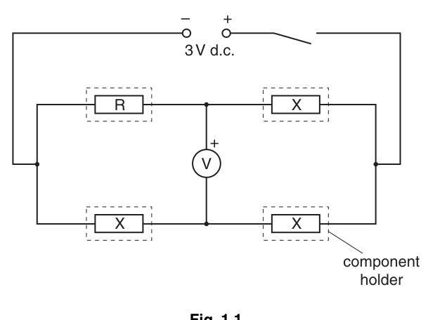
Set up the circuit of Fig. 1.1. The resistor R should have a resistance $R$ where $R = 2.2\text{ k}\Omega$ .

Fig. 1.1

DifficultyEasy

Worked solution

Answer

Circuit connected as in Fig. 1.1 with $R = 2.2\ \text{k}\Omega$ in the correct position and the voltmeter across the central branch with correct polarity.

Final answer

Circuit correctly set up (including R = 2.2 kΩ and correct voltmeter connection).

Detailed explanation

Background Concept

In a resistor network, the potential difference (p.d.) between two points depends on how current divides and how voltages are shared in series/parallel sections. A voltmeter measures the p.d. between two nodes and must be connected in parallel with the part of the circuit being measured. It also has polarity: a positive reading means the terminal marked "+" is at higher potential than the other terminal.

Understanding the Question

You are given a circuit diagram (Fig. 1.1) showing a 3 V d.c. supply, a switch, a diamond/bridge arrangement of resistors (one labelled $R$ and three labelled $X$ ), and a voltmeter connected across the central vertical branch (with the positive voltmeter terminal at the top). You must build this circuit with $R = 2.2\ \text{k}\Omega$ .

Approach

Place the resistors exactly in the positions shown (especially the single resistor labelled $R$ ).
Connect the voltmeter across the correct two nodes (the two points of the central vertical branch), not in series.
Check polarity of the voltmeter and ensure the supply and switch are in the correct places before closing the switch.

Step-by-Step Reasoning

diagram-1a

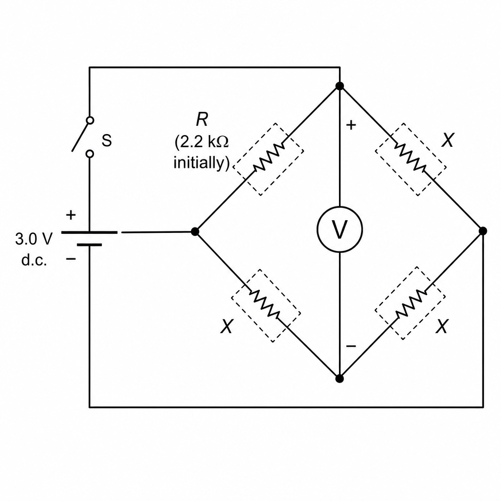
Identify the four sides of the bridge/diamond and place the resistor labelled $R$ at the top-left position as shown.
Place the three identical resistors labelled $X$ in the remaining three positions.
Connect the 3 V supply across the left and right nodes of the bridge network (as in the diagram) with the switch in series.
Connect the voltmeter between the top junction and the bottom junction of the central vertical branch. The top junction must go to the positive voltmeter terminal so that a higher potential at the top gives a positive $V$ .
Only when all connections are secure do you close the switch.

Key Takeaways

Voltmeters are connected in parallel across two nodes.
Correct polarity matters when negative readings are possible.
Practical marks often reward building exactly what the diagram shows.

Common Mistakes

Connecting the voltmeter in series (gives incorrect readings and can disrupt the circuit).
Putting $R$ in the wrong arm of the network (changes the whole relationship between $V$ and $R$ ).
Reversing voltmeter leads so the sign of $V$ is opposite to expectation.

Things to Be Careful About

$R$ is specified as $2.2\ \text{k}\Omega$ here; do not use $2.2\ \Omega$ .
Ensure firm connections in the component holder to avoid intermittent contact.
Keep the switch open while changing resistors to prevent heating and drifting readings.

Techniques used

assemble a circuit exactly as shown in the circuit diagramcheck polarity and correct connection of the voltmeter in parallelverify component values before switching on

(b)

Close the switch and record the voltmeter reading $V$ , which should be in the range $+0.10\text{ V}$ to $+0.90\text{ V}$ .
Open the switch.

$V$ = ______ $\text{V}$

DifficultyEasy

Worked solution

Answer

(Example within the required range)

$V = +0.63\ \text{V}$

Final answer

V = +0.63 V (example; student-dependent)

Detailed explanation

Background Concept

A voltmeter measures the potential difference between two points. Because it has very high resistance, it draws negligible current and should not significantly change the circuit. The reading can be positive or negative depending on which terminal is at higher potential.

Understanding the Question

With $R = 2.2\ \text{k}\Omega$ in place, you close the switch, read the voltmeter value $V$ (expected between $+0.10\ \text{V}$ and $+0.90\ \text{V}$ ), then open the switch. The mark is for a sensible recorded value and correct use of sign/unit.

Approach

Close the switch only long enough to obtain a steady reading.
Record the voltmeter reading including the sign.
Write the value to the resolution of the meter (e.g. to 0.01 V if a digital meter shows 2 d.p.).

Step-by-Step Reasoning

Ensure the voltmeter is on a suitable range (e.g. 0–2 V or 0–20 V d.c.).
Close the switch and wait briefly for the reading to stabilise.
Read and record $V$ with unit V (and a plus sign if the meter indicates it).
Open the switch after taking the reading.

A typical value (consistent with the required range) is $V = +0.63\ \text{V}$ .

Key Takeaways

Always include unit and sign for p.d.
Keep the circuit on only as long as needed to avoid heating effects.

Common Mistakes

Forgetting the unit (V) or omitting the sign.
Recording an unstable reading (not allowing the meter to settle).
Leaving the switch closed for long periods so resistors warm up and readings drift.

Things to Be Careful About

If the voltmeter connections are reversed, the magnitude may be similar but the sign will change.
If the value is outside the given range, re-check the circuit and that $R$ really is $2.2\ \text{k}\Omega$ .

Techniques used

measure potential difference using a voltmeter connected in parallelrecord a reading with appropriate sign and resolutionopen the switch between measurements to prevent heating

(c)

(i)

Change resistor R for one of another value. Close the switch and record the new resistance $R$ and the voltmeter reading $V$ .
Open the switch.

$R$ = ______ $\text{k}\Omega$
$V$ = ______ $\text{V}$

DifficultyMedium-Easy

Worked solution

Answer

(Example readings)

$R = 1.00\ \text{k}\Omega$

$V = +0.40\ \text{V}$

Final answer

R = 1.00 kΩ, V = +0.40 V (example; student-dependent)

Detailed explanation

Background Concept

To investigate how $V$ depends on $R$ , you vary only $R$ (independent variable) and measure the resulting $V$ (dependent variable) while keeping the rest of the circuit unchanged. This is a controlled experiment: changing one quantity at a time helps ensure any change in $V$ is due to $R$ .

Understanding the Question

You must replace resistor $R$ with a different value, then (with the switch closed briefly) record the new value of $R$ and the corresponding voltmeter reading $V$ . The values must be recorded with units ( $\text{k}\Omega$ for $R$ , V for $V$ ).

Approach

Open the switch before changing $R$ .
Choose a resistor with a different stated value (or measure it if required).
Close the switch and record the new $V$ .

Step-by-Step Reasoning

With the switch open, remove the $2.2\ \text{k}\Omega$ resistor and insert another resistor into the same position.
Record the resistance value $R$ (in $\text{k}\Omega$ ) from the label or from an ohmmeter if provided.
Close the switch and read the voltmeter; record $V$ including sign.
Open the switch again.

Example: $R = 1.00\ \text{k}\Omega$ , $V = +0.40\ \text{V}$ .

Key Takeaways

Vary the independent variable ( $R$ ) and measure the dependent variable ( $V$ ).
Keep the circuit configuration identical for each run.

Common Mistakes

Changing the wrong resistor (an $X$ resistor instead of $R$ ).
Forgetting to open the switch before changing components.
Recording $R$ in $\Omega$ instead of $\text{k}\Omega$ .

Things to Be Careful About

Use a sensible range of $R$ values across the six readings overall (small to large) to produce a clear trend on the graph.
Ensure good electrical contact in the holder; poor contact causes fluctuating $V$ .

Techniques used

replace a component while keeping the rest of the circuit unchangedmeasure resistance value and corresponding potential differencerecord measurements with correct units and precision

(ii)

Repeat (c)(i) until you have six sets of readings for $R$ (in $\text{k}\Omega$ ) and $V$ . Include in your table of results values for $\frac{R}{R + 1}$ , where $R$ is in $\text{k}\Omega$ .

Some resistors may give negative values for $V$ .

11M

DifficultyMedium

Worked solution

Answer

Record six sets of readings of $R$ (in $\text{k}\Omega$ ) and $V$ (in V) and calculate $\dfrac{R}{R+1}$ for each row.

Example of a correctly laid-out table (values are illustrative):

$R / \text{k}\Omega$	$V / \text{V}$	$\dfrac{R}{R+1}$
0.10	$-0.09$	0.091
0.22	$+0.02$	0.180
0.47	$+0.18$	0.320
1.00	$+0.40$	0.500
2.20	$+0.63$	0.688
4.70	$+0.79$	0.825

Final answer

Six readings of R and V recorded in one table, with calculated R/(R+1) column (student-dependent values).

Detailed explanation

Background Concept

Good practical data must be:

Sufficient in quantity (enough points to show a trend).
Spread over a suitable range of the independent variable.
Recorded clearly with units and consistent precision.

When a graph requires a derived quantity (here $\dfrac{R}{R+1}$ ), you calculate it for each row using the measured $R$ values. Since $R$ is specified to be in $\text{k}\Omega$ , the calculation must use $R$ in $\text{k}\Omega$ so that the "+1" corresponds to $1\ \text{k}\Omega$ .

Understanding the Question

You must take six pairs of readings $(R, V)$ by changing $R$ each time, then produce a results table including a calculated column for

\frac{R}{R+1}

The question warns that some $V$ values may be negative, so your table (and later graph) must allow for negative $V$ .

Approach

Choose at least six different values of $R$ spanning a good range (including small and large values) to make $\dfrac{R}{R+1}$ vary significantly.
For each $R$ , measure/record $V$ with the correct sign.
Compute $\dfrac{R}{R+1}$ for each row and record it to a sensible number of decimal places (often 3 d.p. is adequate for plotting).
Present all data in one clear table with headings containing quantity and unit.

Step-by-Step Reasoning

Decide on six resistor values (e.g. 0.10, 0.22, 0.47, 1.0, 2.2, 4.7 k\Omega).
For each value:
- switch open (\rightarrow) change resistor (\rightarrow) switch closed briefly (\rightarrow) read $V$ (\rightarrow) switch open.
- record $R$ in $\text{k}\Omega$ and $V$ in V.
Calculate the derived column using the exact recorded $R$ :

\frac{R}{R+1}

Example calculations:

If $R = 2.20\ \text{k}\Omega$ ,

\frac{R}{R+1} = \frac{2.20}{2.20+1.00} = \frac{2.20}{3.20} = 0.688

If $R = 0.10\ \text{k}\Omega$ ,

\frac{R}{R+1} = \frac{0.10}{1.10} = 0.091

Then record all six rows in a single table with clear headings and consistent decimal places for $V$ .

Key Takeaways

A good range of $R$ values produces a better graph.
Derived columns must be calculated correctly and consistently.
Negative readings must be recorded, not ignored.

Common Mistakes

Using $R$ in $\Omega$ when calculating $\dfrac{R}{R+1}$ (the "+1" would then be wrong by a factor of 1000).
Missing units in the headings (e.g. writing just $R$ and $V$ ).
Inconsistent precision within a column (e.g. mixing 0.4, 0.40, 0.402).
Rounding $\dfrac{R}{R+1}$ too aggressively (e.g. to 1 d.p.), which makes the graph less accurate.

Things to Be Careful About

Keep the switch open between readings to reduce heating.
Ensure resistor values are clearly identified; if they are close in value, label them or measure with a meter if available.
Include a wide enough spread so the plotted $x$ -values are not all clustered together.

Techniques used

collect a suitable range of paired readings while varying one variablerecord all results in a single table with correct headings and unitscalculate a derived quantity for each rowinclude negative readings where appropriate

(d)

(i)

Plot a graph of $V$ on the $y$ -axis against $\frac{R}{R + 1}$ on the $x$ -axis.

DifficultyMedium-Easy

Worked solution

Answer

Plot $V$ on the $y$ -axis against $\dfrac{R}{R+1}$ on the $x$ -axis.

Axes labelled: $V / \text{V}$ and $\dfrac{R}{R+1}$ .
Sensible scales using most of the grid.
Plot all six points accurately (including any negative $V$ ).

Final answer

Graph of V (y) against R/(R+1) (x) with correct labels/scales and all points plotted.

Detailed explanation

Background Concept

A graph is used to reveal relationships between variables. If you plot the correct variables and the relationship is linear, the points should lie close to a straight line. Good graph technique is assessed in Paper 3: correct axis choice, clear labels, sensible scales, and accurate plotting.

Understanding the Question

You are told explicitly what to plot:

vertical axis: $V$
horizontal axis: $\dfrac{R}{R+1}$

Your table from (c)(ii) provides these values. Some $V$ values may be negative, so your $y$ -axis scale must include negative values if needed.

Approach

Put the independent variable on the $x$ -axis: $\dfrac{R}{R+1}$ .
Put the dependent variable on the $y$ -axis: $V$ .
Choose scales that use at least half (ideally most) of the grid in both directions.
Plot each point with a small, neat cross or dot.

Step-by-Step Reasoning

Draw axes and label them:
- $x$ -axis: $\dfrac{R}{R+1}$ (dimensionless, so no unit needed).
- $y$ -axis: $V / \text{V}$ .
Decide the range:
- $\dfrac{R}{R+1}$ is between 0 and 1, so a typical range might be 0.05 to 0.90 depending on your data.
- $V$ should include your lowest and highest readings; if any are negative, include a negative section.
Plot all six points from your table accurately.

Key Takeaways

Correct variables on correct axes is essential.
A good scale improves accuracy when drawing the best-fit line and finding gradient.

Common Mistakes

Plotting $R$ instead of $\dfrac{R}{R+1}$ .
Forgetting to label axes with quantity and unit (especially $V / \text{V}$ ).
Using a cramped scale that uses only a small part of the grid.

Things to Be Careful About

Do not force the graph to start at zero unless it suits your data.
If negative $V$ occurs, extend the $y$ -axis below zero rather than omitting points.

Techniques used

label axes with correct variables and unitschoose a suitable scale that uses most of the graph gridplot points accurately including negative values where present

(ii)

Draw the straight line of best fit.

DifficultyEasy

Worked solution

Answer

Draw one straight line of best fit through the plotted points (balanced scatter about the line).

Final answer

Straight line of best fit drawn.

Detailed explanation

Background Concept

When data should follow a linear relationship, experimental scatter means points will not lie perfectly on a line. The best-fit line represents the trend: it should pass as close as possible to the points with roughly equal numbers above and below.

Understanding the Question

After plotting $V$ against $\dfrac{R}{R+1}$ , you must draw the straight line that best represents the trend of all six points.

Approach

Use a ruler.
Do not join dot-to-dot.
Aim for a line that balances the scatter rather than passing through every point.

Step-by-Step Reasoning

Inspect the distribution of points.
Place the ruler so that the line is as close as possible to all points.
Adjust so that the points are roughly balanced above and below the line along its length.
Draw a single continuous straight line across the full range of the data.

Key Takeaways

A best-fit line is a trend line, not a connection between points.

Common Mistakes

Drawing a line through the first and last point regardless of the rest.
Drawing multiple short segments instead of one straight line.

Things to Be Careful About

If there is one clear anomalous point, do not force the line to pass through it; still balance the majority of points (unless instructed otherwise).

Techniques used

judge the overall trend of the plotted pointsdraw a single straight line of best fit with balanced scatter

(iii)

Determine the gradient and $y$ -intercept of this line.

gradient = ______
$y$ -intercept = ______

DifficultyMedium-Easy

Worked solution

Working

Use a large triangle on the best-fit line:

\text{gradient} = \frac{\Delta V}{\Delta\left(\frac{R}{R+1}\right)}

Read the $y$ -intercept at $\dfrac{R}{R+1} = 0$ .

(Example values)

gradient $= 1.20$

$y$ -intercept $= -0.20\ \text{V}$

Answer

gradient $= 1.20$

$y$ -intercept $= -0.20\ \text{V}$

Final answer

gradient = 1.20, y-intercept = −0.20 V (example; student-dependent)

Detailed explanation

Background Concept

For a straight-line graph, the gradient is the rate of change of $y$ with respect to $x$ :

\text{gradient} = \frac{\Delta y}{\Delta x}

The $y$ -intercept is the value of $y$ where $x = 0$ . Using a large triangle reduces percentage reading uncertainty because the same absolute reading error is a smaller fraction of a larger (\Delta x) and (\Delta y).

Understanding the Question

You have drawn a best-fit straight line on a graph of $V$ (y-axis) against $\dfrac{R}{R+1}$ (x-axis). You must find:

gradient of the best-fit line
$y$ -intercept of the best-fit line

Approach

Choose two well-separated points on the best-fit line (not necessarily actual plotted points).
Read off their coordinates and compute the gradient using $\Delta V / \Delta x$ .
Extend the best-fit line to the $y$ -axis (where $x=0$ ) and read the intercept.

Step-by-Step Reasoning

Pick two points far apart on the line, e.g. at $x_1$ and $x_2$ .
Read the corresponding $V_1$ and $V_2$ .
Calculate:

\text{gradient} = \frac{V_2 - V_1}{x_2 - x_1}

Here $x$ is dimensionless, so the gradient has units of volts.

For the $y$ -intercept, locate where the best-fit line crosses $x=0$ and read $V$ at that point.

Illustrative example from a typical straight-line plot:

gradient $\approx 1.20$
$y$ -intercept $\approx -0.20\ \text{V}$

Key Takeaways

Use a large triangle for a more accurate gradient.
Gradient is always $\Delta y / \Delta x$ , not $y/x$ .
Intercept is taken from the best-fit line, not from a single data point.

Common Mistakes

Using two nearby points, giving a large uncertainty in gradient.
Calculating $\Delta x / \Delta y$ (inverting the gradient).
Reading the intercept from the nearest plotted point instead of the best-fit line.

Things to Be Careful About

Make sure you use the best-fit line, not a line drawn through points arbitrarily.
If your axes do not include $x=0$ on the visible grid, you must extend the line carefully to estimate the intercept.
Quote the intercept with unit V and include the sign.

Techniques used

determine the gradient using a large triangle on the best-fit lineread the y-intercept from the graph at x = 0use consistent units when calculating gradient

(e)

The relationship between $V$ and $R$ is

V = a \left( \frac{R}{R + 1} \right) - b

where $a$ and $b$ are constants, and $R$ is in $\text{k}\Omega$ .

Using your answers from (d)(iii), determine the values of $a$ and $b$ .
Give an appropriate unit for $b$ .

$a$ = ______
$b$ = ______

DifficultyMedium-Easy

Worked solution

Working

Given

V = a\left(\frac{R}{R+1}\right) - b

Compare with $V = mx + c$ where $x = \dfrac{R}{R+1}$ :

a = \text{gradient}

-b = y\text{-intercept} \Rightarrow b = -\,(y\text{-intercept})

Using (d)(iii) (example): gradient $= 1.20$ , $y$ -intercept $= -0.20\ \text{V}$ ,

a = 1.20

b = -(-0.20\ \text{V}) = 0.20\ \text{V}

Answer

$a = 1.20$

$b = 0.20\ \text{V}$

Final answer

a = gradient; b = −(y-intercept), unit of b is V (example: a = 1.20, b = 0.20 V).

Detailed explanation

Background Concept

A straight-line graph follows

y = mx + c

where $m$ is the gradient and $c$ is the $y$ -intercept. If your experimental plot is $V$ (as $y$ ) against $\dfrac{R}{R+1}$ (as $x$ ), then you can identify constants by comparing the given relationship to this form.

Understanding the Question

You are told that

V = a\left(\frac{R}{R+1}\right) - b

and you have already found the gradient and $y$ -intercept of the graph of $V$ against $\dfrac{R}{R+1}$ . You must determine $a$ and $b$ and give an appropriate unit for $b$ .

Approach

Treat $x = \dfrac{R}{R+1}$ .
Compare the given equation with $V = mx + c$ .
Identify $a$ with $m$ and identify $-b$ with $c$ .
Decide units: since $V$ is in volts and $x$ is dimensionless, $a$ has unit V and $b$ has unit V.

Step-by-Step Reasoning

Rewrite conceptually as:

V = a x - b

where

x = \frac{R}{R+1}

Compare with $V = mx + c$ :

Gradient $m = a$
Intercept $c = -b$

So:

a = \text{gradient}

and

b = -c = -\,(y\text{-intercept})

Example: if the best-fit line has gradient $1.20$ and $y$ -intercept $-0.20\ \text{V}$ then

a = 1.20

b = -(-0.20\ \text{V}) = 0.20\ \text{V}

Unit of $b$ is V because it is subtracted directly from $V$ .

Key Takeaways

Identify constants by matching to $y = mx + c$ .
The sign matters: here $b$ is the negative of the $y$ -intercept.
Units come from the equation: quantities added/subtracted must have the same unit.

Common Mistakes

Stating $b$ equals the $y$ -intercept instead of $b = -\,(y\text{-intercept})$ .
Giving no unit for $b$ or giving the wrong unit.
Confusing the plotted variable ( $x = \dfrac{R}{R+1}$ ) with $R$ itself.

Things to Be Careful About

Keep the sign of the intercept: if the intercept is negative, $b$ becomes positive.
Quote $b$ to a sensible number of significant figures consistent with how precisely the intercept can be read from the graph.

Techniques used

match a linear relationship to y = mx + cidentify constants from gradient and interceptassign correct units to constants from the equation

The rest of this paper

1 more questions

Q2Manipulation, Measurement and Observation · Analysis, Conclusions and Evaluation · Presentation of Data and Observations20M

Loading the full paper…