Physics 9702/33 — May/June 2010

Cambridge AS Level · Advanced Practical Skills · worked solutions for every part, with the mark scheme

questions

120

minutes

Topics Manipulation, Measurement and Observation · Presentation of Data and Observations · Analysis, Conclusions and Evaluation

Q1Manipulation, Measurement and ObservationPresentation of Data and ObservationsAnalysis, Conclusions and EvaluationFree sample

In this experiment, you will investigate how the current through a semiconductor diode depends on the voltage across it.

You may not need to use all of the materials provided.

(a)

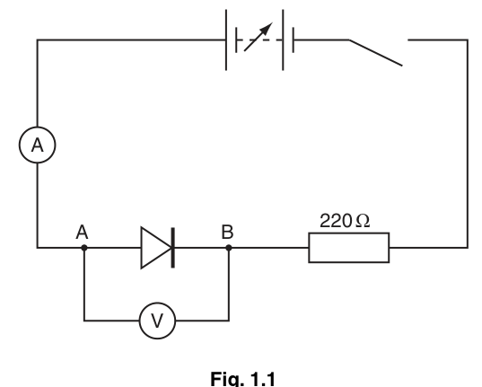
Assemble the circuit of Fig. 1.1.
Make sure that the diode is connected the correct way round.

Fig. 1.1

DifficultyMedium-Easy

Worked solution

Answer

Connect the d.c. supply, switch, $220\ \Omega$ resistor, diode and ammeter all in series.

Connect the voltmeter in parallel across the diode terminals $A$ and $B$ .

Ensure the diode is forward biased (anode to the more positive side of the supply).

Final answer

Series circuit with ammeter in series, voltmeter across diode, diode forward biased.

Detailed explanation

Background Concept

In a circuit diagram:

Components drawn in one loop are in series (same current through each).
A voltmeter must be connected in parallel with the component whose potential difference (p.d.) you are measuring.
An ammeter must be connected in series so the circuit current flows through it.

A semiconductor diode conducts significantly only when forward biased (anode at higher potential than cathode). A series resistor is used to limit the current and protect the diode.

Understanding the Question

You are asked to build the circuit shown and, crucially, connect the diode the correct way round so that a measurable forward current flows when the supply is set to $12\ \text{V}$ .

Approach

Follow the diagram systematically:

Make one complete series loop (supply (\to) switch (\to) resistor (\to) diode (\to) ammeter (\to) back to supply).
Place the voltmeter across the diode terminals only.
Choose the diode orientation that produces forward bias.

Step-by-Step Reasoning

diagram-1a

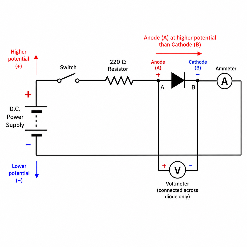
Put the resistor in series with the diode: this limits the current even if the diode conducts strongly.
Put the ammeter in series: if it were in parallel it would (attempt to) take a very large current and could be damaged.
Put the voltmeter across the diode: a voltmeter has a very large resistance, so in parallel it measures p.d. without significantly changing the current.
Check the diode direction: forward bias means the diode’s anode is at the higher potential end of the diode.

Key Takeaways

Ammeter: series; Voltmeter: parallel.
Forward bias is needed for appreciable diode current.
A series resistor protects the diode.

Common Mistakes

Putting the voltmeter in series (gives incorrect readings and can prevent current).
Putting the ammeter in parallel (can blow the fuse / damage the meter).
Reversing the diode so it is reverse biased (current stays near zero).

Things to Be Careful About

Check meter polarity so readings are positive.
Ensure the switch is open while assembling to avoid accidental short circuits.
Confirm all connections are secure before closing the switch.

Techniques used

assemble a series circuit from a circuit diagramconnect an ammeter in series and a voltmeter in parallelset the polarity of a diode to achieve forward biascheck component placement before closing the switch

(b)

Set the power supply voltage to $12\ \text{V}$ and close the switch.
Record the voltmeter reading $V$ and the ammeter reading $I$ .
You should find that $I$ is at least $0.02\ \text{A}$ .

$V$ = ______
$I$ = ______

DifficultyMedium-Easy

Worked solution

Answer

(Example readings)

$V = 0.75\ \text{V}$

$I = 0.050\ \text{A}$

Final answer

Example: V = 0.75 V, I = 0.050 A

Detailed explanation

Background Concept

You are measuring:

Current $I$ through the diode using an ammeter (series connection).
Potential difference $V$ across the diode using a voltmeter (parallel connection).

For a forward-biased diode, the current increases rapidly once the p.d. across it reaches around (0.6)–(0.8\ \text{V}) (typical silicon diode). The series resistor limits the current.

Understanding the Question

With the supply set to $12\ \text{V}$ and the switch closed, you must record one pair of readings $(V, I)$ such that the current is at least $0.02\ \text{A}$ .

Approach

Set the supply to $12\ \text{V}$ .
Close the switch.
Read the voltmeter across the diode and the ammeter in series.
Record both readings with appropriate precision.

Step-by-Step Reasoning

With a $220\ \Omega$ resistor in series, the current is limited to a safe value.
The diode forward p.d. will usually be less than $1\ \text{V}$ even when the supply is $12\ \text{V}$ ; most of the supply voltage appears across the resistor.
Therefore a typical reading might be $V \approx 0.7\text{–}0.8\ \text{V}$ and $I \approx 0.02\text{–}0.06\ \text{A}$ .

Key Takeaways

Record $V$ across the diode, not the supply.
A large supply voltage does not mean a large diode p.d. because of the series resistor.

Common Mistakes

Recording the supply voltage instead of the diode voltage.
Reading the wrong scale or missing the ammeter unit (mA vs A).
Forgetting to include units or using inconsistent decimal places.

Things to Be Careful About

Avoid parallax when reading analogue meters.
Ensure the supply is stable before taking the reading.
If $I < 0.02\ \text{A}$ at $12\ \text{V}$ , the diode may be reversed or there is a poor connection.

Techniques used

set the power supply to a specified valuetake simultaneous readings of current and potential differencerecord readings to an appropriate instrument resolution

(c)

Reduce the power supply voltage, recording $V$ and $I$ until you have six sets of readings.

Open the switch when you have finished your measurements.

Include in your table of results the values of $V^{10}$ .
( $V^{10} = V \times V \times V \times V \times V \times V \times V \times V \times V \times V$ )

DifficultyMedium

Worked solution

Answer

Obtain six sets of readings of $V$ and $I$ as the supply voltage is reduced, and calculate $V^{10}$ for each reading.

(Example of a correctly set-out table)

$V\ /\ \text{V}$	$I\ /\ \text{A}$	$V^{10}\ /\ \text{V}^{10}$
0.75	0.050	0.0563
0.70	0.024	0.0282
0.65	0.011	0.0135
0.60	0.004	0.00605
0.58	0.002	0.00430
0.55	0.001	0.00253

Open the switch after measurements.

Final answer

Six readings of V and I recorded with a V^10 column (values student-dependent).

Detailed explanation

Background Concept

A good results table:

Has a single table containing all readings.
Uses clear headings of the form “quantity / unit”.
Uses consistent decimal places for raw measurements (based on meter resolution).
Includes calculated quantities (here $V^{10}$ ) to a sensible number of significant figures.

Because $V^{10}$ is very sensitive to small changes in $V$ , rounding $V$ too aggressively (e.g. to 1 d.p.) can cause large fractional errors in $V^{10}$ .

Understanding the Question

You must reduce the supply voltage and record $V$ (across the diode) and $I$ (through the diode) until you have six sets of readings. In the same table, you must also include the calculated value of $V^{10}$ for each row.

Approach

Choose the supply voltage as the variable you adjust.
For each setting, wait briefly for readings to stabilise.
Record $(V, I)$ .
Compute $V^{10}$ using a calculator (or repeated multiplication) and enter it in the table.

Step-by-Step Reasoning

Start from the initial setting (near $12\ \text{V}$ supply), where the diode current is clearly measurable.
Decrease the supply in steps so that the diode p.d. and current decrease smoothly; aim for a good spread of $V^{10}$ values (not all clustered).
Record to appropriate resolution (commonly $V$ to $0.01\ \text{V}$ , $I$ to $0.001\ \text{A}$ depending on meter).
Calculate $V^{10}$ . For example, if $V = 0.70\ \text{V}$ then

V^{10} = (0.70)^{10} \approx 0.0282\ \text{V}^{10}.

After finishing, open the switch to avoid heating the diode unnecessarily.

Key Takeaways

Tables must have correct headings/units and consistent precision.
Derived columns (like $V^{10}$ ) must be calculated and recorded clearly.
A good range of the independent variable improves the quality of the graph.

Common Mistakes

Missing units in headings (e.g. writing just $V$ and $I$ ).
Inconsistent decimal places in a single column (suggests poor measurement practice).
Calculating $10V$ instead of $V^{10}$ .
Forgetting to take exactly six sets of readings.

Things to Be Careful About

Do not round $V$ too much before calculating $V^{10}$ ; use the measured value.
Ensure the diode voltage, not the supply voltage, is used for $V^{10}$ .
If using a calculator, check you are using exponentiation correctly ((x^{10}), not (10^x)).

Techniques used

vary the independent variable in steps to obtain a range of readingsrecord results in a table with headings and unitscalculate a derived quantity from measured datause consistent significant figures within each column

(d)

(i)

Plot a graph of $I$ on the $y$ -axis against $V^{10}$ on the $x$ -axis.

DifficultyMedium-Easy

Worked solution

Answer

Plot a graph with:

$y$ -axis: $I\ /\ \text{A}$
$x$ -axis: $V^{10}\ /\ \text{V}^{10}$

Use a suitable scale (at least half the grid in each direction) and plot all six points accurately.

Final answer

Graph of I (A) vs V^10 (V^10), points plotted with suitable scales.

Detailed explanation

Background Concept

A good physics graph should:

Put the stated variables on the correct axes.
Label each axis with “quantity / unit”.
Use a simple, sensible scale (e.g. 1, 2, 5 × powers of ten).
Use most of the available grid to reduce reading uncertainty.
Plot points with small, neat crosses (or dots in circles).

Understanding the Question

You are told exactly what to plot: current $I$ on the $y$ -axis against $V^{10}$ on the $x$ -axis. This is done so you can test whether the data follow a straight-line relationship.

Approach

Decide the axis ranges from your smallest and largest $V^{10}$ and $I$ .
Choose a scale that spreads the points out.
Plot each pair $(V^{10}, I)$ .

Step-by-Step Reasoning

From your table, identify minimum and maximum $V^{10}$ and $I$ .
Mark axes with evenly spaced numbers.
Plot each point carefully; check you have not swapped $x$ and $y$ .

Key Takeaways

Correct axes and good scale choice are worth marks.
Plotting $I$ vs $V^{10}$ is a linearising step.

Common Mistakes

Plotting $V$ instead of $V^{10}$ .
Missing units on axes.
Using an awkward scale (e.g. 3 squares = 0.07) that makes plotting inaccurate.

Things to Be Careful About

Ensure the origin is included only if it fits your data; otherwise start at a suitable value and clearly mark the scale.
Do not join dots point-to-point; you will draw a best-fit line in the next part.

Techniques used

choose appropriate axes for a specified graphlabel axes with quantity and unitplot experimental points accurately with suitable scales

(ii)

Draw the straight line of best fit.

DifficultyMedium-Easy

Worked solution

Answer

Draw a single straight line of best fit through the plotted points so that the points are reasonably balanced above and below the line.

Final answer

Straight line of best fit drawn.

Detailed explanation

Background Concept

A best-fit line represents the overall trend in the data. For experimental scatter, you should not force the line through every point; instead you aim for a line where the vertical deviations are balanced.

Understanding the Question

You must draw the straight line that best represents the relationship between $I$ and $V^{10}$ using your plotted points.

Approach

Use a ruler.
Position the line so that it passes through the “middle” of the points.
Do not automatically force it through the origin unless the pattern clearly requires it.

Step-by-Step Reasoning

Place the ruler and rotate it until the points appear roughly equally distributed above and below.
If one point is clearly anomalous, do not force the line to pass through it.

Key Takeaways

The best-fit line is about the overall trend, not connecting dots.
A good best-fit line makes the gradient/intercept more reliable.

Common Mistakes

Joining points dot-to-dot.
Forcing the line through the origin without justification.
Using a line that passes through only two end points while ignoring most points.

Things to Be Careful About

Draw the line long enough to allow accurate gradient/intercept determination (extend it across most of the graph).

Techniques used

draw a balanced straight line through scattered data pointsignore small random scatter when fitting a trend line

(iii)

Determine the gradient and $y$ -intercept of this line.

gradient = ______
$y$ -intercept = ______

DifficultyMedium

Worked solution

Working

Use a large triangle on the best-fit line:

\text{gradient} = \frac{\Delta I}{\Delta (V^{10})}

(Example from a best-fit line)

\text{gradient} \approx 0.90\ \text{A}\ \text{V}^{-10}

Read $y$ -intercept at $V^{10}=0$ :

y\text{-intercept} \approx -1.0\times 10^{-3}\ \text{A}

Answer

gradient $\approx 0.90\ \text{A}\ \text{V}^{-10}$

$y$ -intercept $\approx -1.0\times 10^{-3}\ \text{A}$

Final answer

Example: gradient ≈ 0.90 A V^-10, y-intercept ≈ −1.0×10^-3 A

Detailed explanation

Background Concept

For a straight-line graph:

y = mx + c

Gradient $m$ is:

m = \frac{\Delta y}{\Delta x}

$y$ -intercept $c$ is the value of $y$ when $x = 0$ .

On a graph of $I$ (y-axis) against $V^{10}$ (x-axis), the gradient has units:

\frac{\text{A}}{\text{V}^{10}} = \text{A}\ \text{V}^{-10}.

Understanding the Question

You must take your best-fit line and find:

Its gradient.
Its $y$ -intercept.

These will be used in the next part to determine constants in a suggested model.

Approach

Choose two well-separated points on the best-fit line (not necessarily actual data points).
Form a large triangle to reduce percentage uncertainty.
Compute (\Delta I) and (\Delta(V^{10})), then divide.
Read the intercept by extending the line to the y-axis (or to $V^{10}=0$ ).

Step-by-Step Reasoning

diagram-1diii

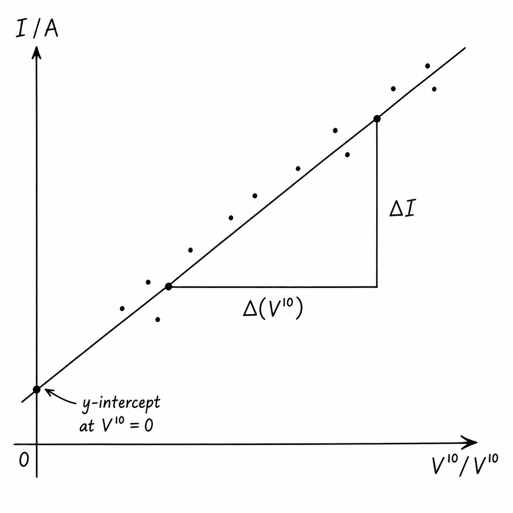
Pick two points far apart on the line, e.g. one near the left and one near the right of the graph.
Read off their coordinates: ((V^{10}_1, I_1)) and ((V^{10}_2, I_2)).
Calculate changes:

\Delta I = I_2 - I_1, \quad \Delta(V^{10}) = V^{10}_2 - V^{10}_1.

Gradient:

\text{gradient} = \frac{\Delta I}{\Delta(V^{10})}.

Extend the best-fit line to $V^{10}=0$ and read the $I$ value there as the $y$ -intercept.

Key Takeaways

Always use a large triangle and points on the best-fit line.
Units of gradient come directly from the axes.

Common Mistakes

Using two nearby points (gives a large uncertainty in gradient).
Using a single data point and the origin to find gradient.
Calculating $\Delta x / \Delta y$ instead of $\Delta y / \Delta x$ .
Forgetting to include units for gradient and intercept.

Things to Be Careful About

Read values from the drawn line, not from the table.
Keep signs correct: if the line intercept is below zero, the intercept is negative.
Make sure the line is extended clearly enough to read the intercept accurately.

Techniques used

determine a gradient using a large triangle on a best-fit lineread a y-intercept from a graphuse correct units from axis labels

(e)

It is suggested that the relationship between $I$ and $V$ is

I = aV^{10} + b

where $a$ and $b$ are constants.

Using your answers from (d)(iii), determine the values of $a$ and $b$ .
Give appropriate units.

$a$ = ______
$b$ = ______

DifficultyMedium-Easy

Worked solution

Working

Given

I = aV^{10} + b

Comparing with $I = m(V^{10}) + c$ gives:

a = \text{gradient}, \quad b = y\text{-intercept}.

Units:

[a] = \frac{\text{A}}{\text{V}^{10}} = \text{A}\ \text{V}^{-10}, \quad [b] = \text{A}.

(Using the example values from (d)(iii))

a \approx 0.90\ \text{A}\ \text{V}^{-10}

b \approx -1.0\times 10^{-3}\ \text{A}

Answer

$a = \text{gradient}$ in $\text{A}\ \text{V}^{-10}$

$b = y$ -intercept in $\text{A}$

Final answer

a = gradient (A V^-10), b = y-intercept (A)

Detailed explanation

Background Concept

If plotting $y$ against $x$ gives a straight line, then the relationship is of the form:

y = mx + c.

Here, the graph is $I$ (y) against $V^{10}$ (x), so the straight-line model is:

I = (\text{gradient})\,V^{10} + (y\text{-intercept}).

Constants’ units come from the equation: the units on both sides must match.

Understanding the Question

You are told the suggested model is:

I = aV^{10} + b.

You have already found the gradient and $y$ -intercept from the $I$ vs $V^{10}$ graph, so you now just identify $a$ and $b$ from those graphical quantities and state appropriate units.

Approach

Recognise it is already linear in $V^{10}$ .
Compare term-by-term with $y = mx + c$ .
Assign $a$ to the gradient and $b$ to the intercept.
Work out the units using dimensional consistency.

Step-by-Step Reasoning

Since the graph is $I$ against $V^{10}$ , the line equation is:

I = m(V^{10}) + c.

Comparing with $I = aV^{10} + b$ gives:

a = m,\quad b = c.

Units:
- $I$ is in $\text{A}$ .
- $V^{10}$ is in $\text{V}^{10}$ .
- Therefore

[a] = \frac{\text{A}}{\text{V}^{10}} = \text{A}\ \text{V}^{-10},

and

[b] = \text{A}.

Key Takeaways

When you plot $I$ vs $V^{10}$ , the gradient corresponds directly to $a$ and the intercept to $b$ .
Always state units for experimentally determined constants.

Common Mistakes

Swapping $a$ and $b$ .
Giving $a$ the wrong unit (e.g. $\text{A V}^{-1}$ instead of $\text{A V}^{-10}$ ).
Writing the intercept as a unitless number.

Things to Be Careful About

Use your own measured gradient/intercept values from (d)(iii); the numerical values depend on your graph.
If your intercept is negative, keep the sign (it may reflect experimental/systematic effects).

Techniques used

match a linear equation to y = mx + cidentify constants from gradient and interceptdeduce units of constants from the equation

The rest of this paper

1 more questions

Q2Manipulation, Measurement and Observation · Analysis, Conclusions and Evaluation · Presentation of Data and Observations

Loading the full paper…