You may not need to use all of the materials provided. In this experiment, you will measure the current through a set of resistors. (i) Connect the circuit of Fig. 1.1, ensuring that the movable lead is connected between resistors 1 and 2. (ii) Close the switch and record the ammeter reading $I$. Open the switch after recording your measurement. $I$ = \_\_\_\_\_\_ $\text{A}$ (b) By adjusting the movable lead, the resistor Z may be connected in series with a number $N$ of…

(a)(i) Circuit connected with movable lead between resistors 1 and 2. · (a)(ii) I ≈ 0.094 A (example) · (b) Six readings of N and I recorded with derived columns 1/I and R=22N (table required). · (c)(i) Graph of R (Ω) vs 1/I (A⁻¹) plotted. · (c)(ii) Straight best-fit line drawn. · (c)(iii) gradient and y-intercept read from best-fit line (example: 3.00 Ω·A, −10 Ω) · (d) G = gradient (V), H = y-intercept (Ω) (example: 3.00 V, −10 Ω)

Physics 9702/32 — May/June 2010

Cambridge AS Level · Advanced Practical Skills · worked solutions for every part, with the mark scheme

questions

marks

120

minutes

Topics Manipulation, Measurement and Observation · Analysis, Conclusions and Evaluation · Presentation of Data and Observations

Q1Manipulation, Measurement and ObservationPresentation of Data and ObservationsAnalysis, Conclusions and EvaluationFree sample

You may not need to use all of the materials provided.

In this experiment, you will measure the current through a set of resistors.

(a)

(i)

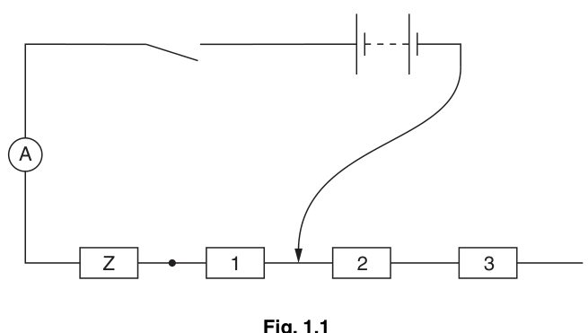
Connect the circuit of Fig. 1.1, ensuring that the movable lead is connected between resistors 1 and 2.

Fig. 1.1

DifficultyMedium-Easy

Worked solution

Answer

Connect the circuit as in Fig. 1.1 with the ammeter in series.
Ensure the movable lead is connected at the junction between resistors 1 and 2 (so resistor Z and resistor 1 are included in series, and resistors 2 and 3 are excluded for this setting).

Final answer

Circuit connected with movable lead between resistors 1 and 2.

Detailed explanation

Background Concept

In a series circuit, the same current flows through every component in the single loop. An ammeter is used to measure current and must be connected in series so that the circuit current passes through it. Ammeter polarity matters: current should enter the ammeter at its positive terminal to give a positive reading.

The “movable lead” acts like a selectable connection point (a tap) along a chain of resistors. By choosing where it connects, you change how many resistors are included in the series path, changing the total resistance and therefore the current.

Understanding the Question

You are asked to build the circuit exactly as shown, with one specific instruction: the movable lead must connect between resistors 1 and 2. That instruction determines which resistors are actually in the current path for part (a).

Approach

Follow the diagram to make one complete loop (cells → switch → ammeter → resistors → back to cells).
Put the movable lead on the correct junction (between 1 and 2), because that selects the resistors included.
Before closing the switch, check all connections are secure and that the ammeter is not bypassed.

Step-by-Step Reasoning

diagram-a-i

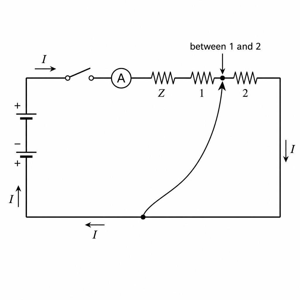
Connect the two cells in series to make the supply.
Connect the switch in series so it can open/close the circuit.
Connect the ammeter in series after the switch (as drawn).
Connect the resistors in the order shown (Z then 1 then 2 then 3, etc. as provided).
Connect the movable lead specifically to the node between resistors 1 and 2. This makes the return path at that node, so the series path includes resistor Z and resistor 1 for this setting.
Check that there is no short circuit (e.g. wires directly across the supply) and that the ammeter is not connected in parallel.

Key Takeaways

Ammeter: always in series, correct polarity.
A movable connection point changes the number of components in series and therefore changes current.
Correctly identifying the junction “between resistors 1 and 2” is essential.

Common Mistakes

Putting the ammeter in parallel (this can blow the fuse / give nonsense readings).
Connecting the movable lead to the wrong junction (e.g. between Z and 1 or between 2 and 3), changing which resistors are included.
Leaving a loose connection so the circuit is open even when the switch is closed.

Things to Be Careful About

Ensure the ammeter range is suitable before closing the switch (start on a higher current range if available).
Make sure the junction “between 1 and 2” means the node after resistor 1 and before resistor 2.
Avoid heating effects: do not leave the switch closed longer than necessary.

Techniques used

assemble the circuit exactly as shown in the circuit diagramplace the ammeter in series and observe correct polarityposition the movable lead to select the required number of series resistors

(ii)

Close the switch and record the ammeter reading $I$ . Open the switch after recording your measurement.

$I$ = ______ $\text{A}$

DifficultyEasy

Worked solution

Answer

Close the switch, read the ammeter current $I$ , then open the switch.

Example (typical):

I = 0.094\ \text{A}

Final answer

I ≈ 0.094 A (example)

Detailed explanation

Background Concept

Current $I$ is the rate of flow of charge:

I = \frac{\Delta Q}{\Delta t}

An ammeter measures the current through it and must be in series so that the circuit current passes through the meter. In practical work, you record the reading with an appropriate number of decimal places based on the meter’s smallest scale division (or digital resolution).

Understanding the Question

With the circuit set as in (a)(i), you must momentarily close the switch, record the ammeter reading $I$ (in amperes), and then open the switch again.

Approach

Close switch briefly to minimise heating of resistors.
Wait for the reading to settle.
Read the scale/digital display carefully and record the value with correct unit ( $\text{A}$ ).

Step-by-Step Reasoning

Set the ammeter to a suitable range (to avoid overloading). If unsure, start with the highest current range.
Close the switch and allow the pointer/display to stabilise.
Read the ammeter at eye level (analogue) to avoid parallax.
Record $I$ to the meter’s resolution and include the unit $\text{A}$ .
Open the switch immediately after taking the reading to reduce temperature rise (which would change resistance and hence current).

Key Takeaways

Ammeter reading must be recorded with unit and appropriate precision.
Closing the switch only briefly improves reliability by reducing heating.

Common Mistakes

Forgetting the unit $\text{A}$ .
Recording too many/few decimal places (not matching meter resolution).
Leaving the switch closed, allowing resistors to warm up and current to drift.

Things to Be Careful About

If the ammeter has internal fuse protection, exceeding the range may blow the fuse.
On analogue meters, always account for the correct scale and range multiplier.

Techniques used

close the switch only while taking a readingread the ammeter at eye level to avoid parallaxrecord the current to the appropriate resolution

(b)

By adjusting the movable lead, the resistor Z may be connected in series with a number $N$ of other resistors. Each of the resistors labelled 1 to 12 has a resistance of $22\ \Omega$ .

Repeat (a)(ii) for different values of $N$ until you have six sets of readings for $N$ and $I$ .

Include in your table of results values of $\frac{1}{I}$ and the total resistance $R$ of the $22\ \Omega$ resistors connected into the circuit.

(The total resistance $R$ of the $22\ \Omega$ resistors in series can be determined using the formula $R = R_1 + R_2 + R_3 + \dots$ )

DifficultyMedium

Worked solution

Answer

Take six different values of $N$ and measure the corresponding current $I$ each time.
Calculate

\frac{1}{I}\ (\text{A}^{-1})

and

R = 22N\ (\Omega)

Record all values in one results table with headings including units.

Example of a correctly formatted table (values are illustrative):

$N$	$I\ /\ \text{A}$	$1/I\ /\ \text{A}^{-1}$	$R\ /\ \Omega$
1	0.094	10.7	22
2	0.0556	18.0	44
3	0.0395	25.3	66
4	0.0306	32.7	88
5	0.0250	40.0	110
6	0.0211	47.4	132

Final answer

Six readings of N and I recorded with derived columns 1/I and R=22N (table required).

Detailed explanation

Background Concept

For resistors in series, the total resistance is the sum:

R_{\text{series}} = R_1 + R_2 + R_3 + \dots

Here, the identical resistors each have resistance $22\ \Omega$ . If $N$ of them are connected in series, their total resistance is

R = 22N

The question also asks you to compute $1/I$ . This is a standard linearising step because many circuit relationships become straight-line graphs when plotted against reciprocal current.

Understanding the Question

You adjust the movable lead so that resistor Z is in series with a chosen number $N$ of the $22\ \Omega$ resistors (labelled 1 to 12). For each chosen $N$ , you measure the current $I$ . You must obtain six sets of readings and present them in a table, including calculated values of $1/I$ and the total resistance $R$ of the $22\ \Omega$ resistors only.

So, for each row you need:

$N$ (integer)
$I$ (measured)
$1/I$ (calculated)
$R = 22N$ (calculated)

Approach

Choose six different values of $N$ spanning a sensible range (e.g. small to larger $N$ ).
For each $N$ $N$ :
- set the movable lead,
- close switch briefly and measure $I$ ,
- open switch,
- calculate $1/I$ and $R=22N$ .
Present everything in one clear table with units in headings and consistent significant figures.

Step-by-Step Reasoning

Decide on six values of $N$ (for example $N=1$ to $6$ , or spread further if current remains measurable).
For each $N$ , reposition the movable lead to include exactly $N$ of the $22\ \Omega$ resistors in the series path with Z.
Measure $I$ $I$ :
- close switch,
- wait for stable reading,
- record $I$ to the meter resolution,
- open switch.
Calculate the derived columns:
- Reciprocal current: $\frac{1}{I}$ Units: $\text{A}^{-1}$ .
- Total resistance of the $22\ \Omega$ resistors: $R = 22N$ Units: $\Omega$ .
Table presentation:
- Put units in the column headings (not next to every number).
- Keep consistent decimal places in the $I$ column (to match meter resolution) and consistent significant figures in $1/I$ .
- Ensure you actually have six complete rows.

Key Takeaways

Series resistances add; identical resistors give $R=22N$ .
Derived quantities ( $1/I$ and $R$ ) must be calculated and tabulated correctly.
Good tables have clear headings with units and consistent precision.

Common Mistakes

Using $R=\frac{22}{N}$ (wrong for series; that would resemble parallel reasoning).
Forgetting to include units in headings.
Mixing precision (e.g. some $I$ values to 1 d.p., others to 3 d.p.) without justification.
Calculating $1/I$ with incorrect rounding or using inconsistent significant figures.

Things to Be Careful About

$R$ here is only the total of the $22\ \Omega$ resistors, not including resistor Z.
If the current becomes very small for large $N$ , choose a range of $N$ where readings are still reliable (avoid values near the meter’s noise/zero drift).

Techniques used

vary the independent variable systematically to obtain a suitable rangecalculate derived quantities from measured valuesrecord results in a single table with correct headings and unitsmaintain consistent significant figures within each column

(c)

(i)

Plot a graph of $R$ on the $y$ -axis against $\frac{1}{I}$ on the $x$ -axis.

DifficultyMedium-Easy

Worked solution

Answer

Plot $R\ (\Omega)$ on the $y$ -axis against $1/I\ (\text{A}^{-1})$ on the $x$ -axis.
Use a scale that uses at least half the grid in both directions and plot all six points as small crosses.

Final answer

Graph of R (Ω) vs 1/I (A⁻¹) plotted.

Detailed explanation

Background Concept

A graph is used to reveal patterns and allow constants to be found from a straight-line relationship. Correct graphing conventions (labels, units, sensible scales, accurate plotting) are assessed directly in Paper 3.

Understanding the Question

You have calculated columns for $R$ and $1/I$ . You must make a graph with:

vertical axis: $R$
horizontal axis: $1/I$

This specific choice of axes is important because later parts use the gradient and intercept.

Approach

Put the stated variable on each axis (do not swap).
Use an easy-to-read linear scale.
Plot six points accurately.

Step-by-Step Reasoning

Draw axes and choose scales:
- Let $x$ run from slightly below the smallest $1/I$ to slightly above the largest $1/I$ .
- Let $y$ run from slightly below the smallest $R$ to slightly above the largest $R$ .
- Avoid awkward scales (e.g. 3 squares = 1 unit).
Label axes with quantity and unit:
- $x$ -axis: $1/I\ /\ \text{A}^{-1}$
- $y$ -axis: $R\ /\ \Omega$
Plot each data pair $(1/I, R)$ as a small cross (×) with a consistent symbol size.

Key Takeaways

Correct axis assignment and correct labels (with units) are essential.
A good scale uses most of the available grid.

Common Mistakes

Plotting $I$ instead of $1/I$ .
Swapping axes (plotting $1/I$ on $y$ and $R$ on $x$ ).
Missing units in labels.
Using dots that are too large (hiding accuracy) instead of neat crosses.

Things to Be Careful About

Ensure you plot from the calculated $1/I$ values, not from $I$ .
Do not force the graph through the origin unless justified by the data and relationship.

Techniques used

choose appropriate axes and scales that use most of the graph gridlabel axes with quantity and unitplot points accurately from a results table

(ii)

Draw the line of best fit.

DifficultyMedium-Easy

Worked solution

Answer

Draw a single straight line of best fit through the plotted points so that the points are approximately balanced about the line (do not join point-to-point).

Final answer

Straight best-fit line drawn.

Detailed explanation

Background Concept

When data are expected to follow a linear relationship, random uncertainties mean points scatter about the ‘true’ line. A best-fit line is drawn to represent the overall trend, not to pass through every point.

Understanding the Question

After plotting $R$ against $1/I$ , you must draw the line of best fit. This line will be used to find the gradient and intercept, so it must be drawn carefully.

Approach

Use a ruler to draw one straight line.
Aim for an even distribution of points above and below the line.
Ignore small random scatter; do not connect consecutive points.

Step-by-Step Reasoning

Visually judge the trend of the points.
Place a ruler so the line passes through the middle of the cluster of points.
Adjust so that (as far as possible) the number of points above and below are similar and the vertical deviations are of comparable size.
Draw the line across the full range of the data (not just between two points).

Key Takeaways

Best-fit line represents the overall relationship; it is not “join the dots”.
A long line makes gradient/intercept determination more accurate.

Common Mistakes

Joining the points one by one.
Drawing a line through the first and last points only (can be badly affected by outliers).
Drawing a short line segment instead of extending across the data range.

Things to Be Careful About

If one point is a clear anomaly, you still normally draw the best-fit line for the main trend (unless instructed otherwise), but do not force the line to pass through the anomalous point.

Techniques used

draw a single straight line that best represents the trendbalance the line so points are distributed evenly about itavoid join-the-dots and avoid using an endpoint-to-endpoint line

(iii)

Determine the gradient and $y$ -intercept of the line of best fit.

gradient = ______
$y$ -intercept = ______

DifficultyMedium

Worked solution

Working

Using two well-separated points on the best-fit line:

\text{gradient} = \frac{\Delta R}{\Delta(1/I)}

Read the $y$ -intercept $c$ where the line crosses the $R$ -axis.

Example (illustrative):
If two points on the line are $(10.0\ \text{A}^{-1},\ 20\ \Omega)$ and $(45.0\ \text{A}^{-1},\ 125\ \Omega)$ ,

\text{gradient} = \frac{125-20}{45.0-10.0} = 3.00\ \Omega\,\text{A}

and

\text{$y$-intercept} = -10\ \Omega

Answer

gradient $= 3.00\ \Omega\,\text{A}$

$y$ -intercept $= -10\ \Omega$

Final answer

gradient and y-intercept read from best-fit line (example: 3.00 Ω·A, −10 Ω)

Detailed explanation

Background Concept

For a straight-line graph of the form

y = mx + c

the gradient (slope) is

m = \frac{\Delta y}{\Delta x}

the $y$ -intercept is $c$ , the value of $y$ when $x=0$ .

Here, $y$ is $R$ and $x$ is $1/I$ , so:

gradient units are $\Omega$ per $\text{A}^{-1}$ , i.e.

\frac{\Omega}{\text{A}^{-1}} = \Omega\,\text{A} = \text{V}

intercept units are $\Omega$ .

Understanding the Question

You must use your drawn best-fit line (not individual points) to determine:

the gradient of the $R$ vs $1/I$ graph
the $y$ -intercept of that line

These will be used directly in part (d).

Approach

Choose two points far apart on the best-fit line (to reduce percentage reading error).
Read their coordinates $(1/I, R)$ from the axes.
Compute gradient $=\Delta R/\Delta(1/I)$ .
Read the intercept where the best-fit line crosses the $R$ -axis at $1/I=0$ (this may require extrapolation).

Step-by-Step Reasoning

Selecting points:
- Pick points on the line that are easy to read (near grid intersections).
- Ensure they are widely separated in $x$ .
Reading values:
- Read $R$ in $\Omega$ from the y-axis.
- Read $1/I$ in $\text{A}^{-1}$ from the x-axis.
Gradient calculation: $\text{gradient} = \frac{R_2 - R_1}{(1/I)_2 - (1/I)_1}$ Keep units: $\Omega\,\text{A}$ .
Intercept:
- Extend the best-fit line back to $x=0$ .
- Read the corresponding $R$ value; this is the $y$ -intercept (can be negative in this experiment).

Key Takeaways

Always use the best-fit line for gradient/intercept.
Use a large triangle (widely separated points) for better accuracy.
Track units: gradient here has units of voltage.

Common Mistakes

Using two experimental points not on the best-fit line.
Calculating $\Delta x/\Delta y$ instead of $\Delta y/\Delta x$ .
Forgetting that $x$ is $1/I$ (so using $\Delta I$ by mistake).
Giving no units for gradient and intercept.

Things to Be Careful About

If you extrapolate to find the intercept, draw the best-fit line lightly and extend with a ruler; do not guess.
Quote gradient/intercept to a sensible number of significant figures based on graph-reading precision (typically 2–3 s.f.).

Techniques used

use a large triangle on the best-fit line to calculate the gradientcalculate gradient as \Delta y / \Delta x with correct unitsread the y-intercept from where the best-fit line crosses the y-axis

(d)

The quantities $R$ and $I$ are related by the equation

R = \frac{G}{I} + H

where $G$ and $H$ are constants.

Use your answers to (c)(iii) to determine values for $G$ and $H$ . You should include units where appropriate.

$G$ = ______
$H$ = ______

DifficultyMedium-Easy

Worked solution

Working

Given

R = \frac{G}{I} + H

Let $x = 1/I$ , so

R = Gx + H

For the graph of $R$ (y-axis) against $1/I$ (x-axis):

G = \text{gradient},\qquad H = y\text{-intercept}

Units:

[G] = \frac{\Omega}{\text{A}^{-1}} = \Omega\,\text{A} = \text{V},\qquad [H]=\Omega

Answer

$G = 3.00\ \text{V}$

$H = -10\ \Omega$

Final answer

G = gradient (V), H = y-intercept (Ω) (example: 3.00 V, −10 Ω)

Detailed explanation

Background Concept

A straight-line graph is described by

y = mx + c

where $m$ is the gradient and $c$ is the $y$ -intercept.

In this experiment the given relationship is

R = \frac{G}{I} + H

If we define

x = \frac{1}{I}

then the equation becomes

R = Gx + H

which is exactly linear in $x$ .

Understanding the Question

You have already plotted $R$ against $1/I$ and found the gradient and intercept in (c)(iii). This part asks you to interpret those graph quantities as the constants $G$ and $H$ in the given equation, including units.

Approach

Recognise that plotting $R$ (y) against $1/I$ (x) gives a straight line with equation $R = Gx + H$ .
Therefore, identify:
- $G$ as the gradient
- $H$ as the $y$ -intercept
Work out units from the axes.

Step-by-Step Reasoning

Start from $R = \frac{G}{I} + H$
Replace $1/I$ by $x$ : $R = G\left(\frac{1}{I}\right) + H = Gx + H$
Compare with $y=mx+c$ $y = m x + c$ for the graph of $R$ $R$ vs $1/I$ $1/ I$ :
- $y \equiv R$
- $x \equiv 1/I$
- $m \equiv G$
- $c \equiv H$
Units:
- Gradient units are $\frac{\Omega}{\text{A}^{-1}} = \Omega\,\text{A} = \text{V}$ so $G$ is in volts.
- Intercept is a value of $R$ , so $H$ is in ohms.

Key Takeaways

Linearisation: $R = \frac{G}{I}+H$ becomes $R = G(1/I) + H$ .
For a $R$ vs $1/I$ graph, gradient gives $G$ and intercept gives $H$ .
Unit-checking from axes is a powerful validation step.

Common Mistakes

Swapping $G$ and $H$ .
Giving $G$ in $\Omega$ instead of $\text{V}$ .
Using $I$ rather than $1/I$ when matching to $y=mx+c$ .

Things to Be Careful About

If your $y$ -intercept is negative, that can be physically reasonable here because $R$ in the graph excludes resistor Z while the current depends on the total resistance including Z.
Quote $G$ and $H$ to consistent significant figures with your graph results.

Techniques used

match an experimental graph to a linear equation of the form y = mx + cidentify constants from gradient and interceptdeduce correct units from the plotted axes

The rest of this paper

1 more questions

Q2Manipulation, Measurement and Observation · Analysis, Conclusions and Evaluation

Loading the full paper…