Physics 9702/54 — October/November 2025
Cambridge A-Level · Planning, Analysis and Evaluation · worked solutions for every part, with the mark scheme
Topics Analysis, Conclusions and Evaluation · Planning
Fig. 1.1 shows a horizontal turntable.
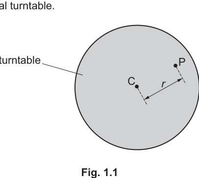
Point C is at the centre of the turntable. Point P is a distance from the centre.
Fig. 1.2 shows a side view of a d.c. motor attached to the turntable with a belt.
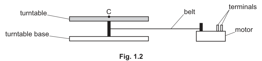
The motor is used to rotate the turntable at frequency . The motor is switched off and the turntable continues to rotate at frequency .
A sphere of adhesive putty of mass is dropped onto the turntable at point P. The frequency of the turntable is now .
It is suggested that is related to by the relationship
where and are constants.
Plan a laboratory experiment to test the relationship between and .
Draw a diagram showing the arrangement of your equipment.
Explain how the results could be used to determine values for and .
In your plan you should include:
- the procedure to be followed
- the measurements to be taken
- the control of variables
- the analysis of the data
- any safety precautions to be taken.
Variables
- Independent variable: mass of adhesive putty added at point .
- Dependent variable: new rotation frequency after putty sticks.
- Controls: radial distance (same marked point ), same turntable and axle, same initial frequency for each run, putty placed so it does not slide, turntable horizontal.
Apparatus and arrangement
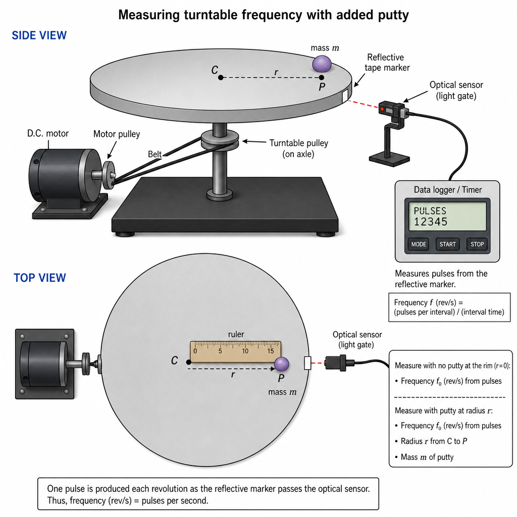
- Turntable driven by d.c. motor and belt.
- Tachometer/optical sensor (or light gate + data logger) to measure frequency using a reflective tape marker on rim.
- Top-pan balance to measure .
- Ruler/set square to mark a fixed radius and the point on the turntable.
Procedure / measurements
- Fix a small reflective strip on the edge of the turntable. Align optical sensor to count one pulse per revolution.
- Mark point at radius from the centre using a ruler; keep constant throughout.
- Prepare several different masses of putty; measure each mass with a balance.
- For one value of :
- Run motor until turntable rotates steadily.
- Switch motor off.
- Immediately measure the frequency just before adding putty, (e.g. measure time for revolutions and use ).
- Drop/place the putty vertically onto point so it sticks with minimal sideways push.
- Measure the new frequency after it settles (again using for the same ).
- Repeat readings for each (at least 5–6 different masses), and repeat each point to obtain mean values.
Analysis (test the relationship; determine and )
Given
Divide by :
So plot against .
- Intercept .
- Gradient , hence
Use a best-fit line and a worst acceptable line to estimate uncertainties in gradient and intercept (hence in and ).
Safety
- Keep fingers/hair/clothing clear of rotating turntable and belt; do not lean over the rotating system.
- Ensure motor is switched off before placing the putty; stand to the side in case putty detaches.
- Secure the motor/turntable so it cannot move on the bench.
See working
Background Concept
When an object rotates, adding a mass at a distance from the axis increases the system’s moment of inertia. If external torque is negligible during the brief “sticking” event, angular momentum is approximately conserved, so the rotation rate decreases.
In this question, you are not asked to derive the relationship; you are asked to test the suggested relationship experimentally and use data to find constants.
The given suggested relationship is
where:
- is the turntable frequency just before the putty is added (motor switched off),
- is the frequency after the putty sticks,
- is the putty mass,
- is the distance of the putty from the centre,
- and are constants for the apparatus.
A key experimental skill here is to rearrange to a linear form so you can use a straight-line graph to test the model and extract constants.
Understanding the Question
You must design a practical method in which you:
- Vary (use different putty masses),
- Measure and for each while keeping the same,
- Analyse results so that if the relationship is correct, your graph is a straight line,
- Use the graph’s gradient and intercept to find and .
Because is the frequency with the motor off and just before adding the putty, you should measure for each run (not assume it is identical every time).
Approach
- Choose a reliable way to measure rotational frequency (optical sensor/light gate + data logger, or a tachometer, or a stroboscope). The easiest to justify for Paper 5 is an optical sensor with a reflective marker giving one pulse per revolution.
- Keep constant by marking a point on the turntable at a measured radius.
- Take multiple masses , measure each with a balance, and for each mass measure (immediately before) and (after it sticks).
- Linearise the suggested equation by dividing by to remove the unknown constant from the left-hand side.
- Plot the appropriate graph; use intercept and gradient to determine and . Include uncertainty handling via best-fit and worst-acceptable lines.
Step-by-Step Reasoning
1) Set up the apparatus and frequency measurement
Attach the motor and belt as shown and place a small reflective strip on the rim. Position an optical sensor so that each revolution produces a single pulse.
Measure frequency by timing many revolutions:
- If you count pulses in time , then
Choosing a larger (e.g. or ) reduces the percentage timing uncertainty.
2) Ensure the radius is controlled
Use a ruler (and ideally a set square) to measure a fixed radius from the centre. Mark point clearly. Every run must place the putty at the same point so is constant.
3) Collect data for multiple values of
For each mass :
- Measure using a balance (record to the balance resolution).
- Spin the turntable with the motor until stable.
- Switch the motor off (so the only torques are resistive, and you are consistent with the statement).
- Immediately measure by timing revolutions.
- Drop/place the putty vertically at so it sticks; avoid giving a sideways push because that would add/remove angular momentum.
- Measure the new steady frequency .
- Repeat to get mean values of and for each .
4) Linearise to obtain a straight-line test
Start with
Divide through by :
This is in straight-line form with:
- intercept
- gradient
So you plot against .
5) Determine and from the graph
From the best-fit straight line:
- is the y-intercept.
- If the gradient is , then
To estimate uncertainty:
- Draw a worst acceptable line (steepest/shallowest line still consistent with the scatter or with error bars).
- Find the change in gradient between best and worst line to estimate , and similarly for the intercept to estimate .
- Propagate to using fractional uncertainty: since ,
(If is measured with uncertainty too, include it: so add in fractional terms.)
Key Takeaways
- A good plan states: independent/dependent variables, control variables, apparatus, method, analysis, and safety.
- Linearising an equation to lets you use a straight-line graph to test the relationship and determine constants.
- Measuring frequency accurately often means timing many cycles/revolutions and dividing.
- Constants are extracted from gradient and intercept; uncertainties come from best-fit vs worst-acceptable lines.
Common Mistakes
- Keeping fixed by assumption instead of measuring it each run (friction means it may differ).
- Forgetting to keep constant, or placing putty inconsistently so the effective radius changes.
- Dropping the putty with a sideways push, which changes angular momentum and ruins the test.
- Plotting the wrong graph (e.g. vs directly) so the relationship is not linear and constants cannot be read reliably.
- Not stating how and are obtained from intercept/gradient.
Things to Be Careful About
- Use consistent units: in , in , so has units .
- Ensure the putty sticks and does not slide outward due to rotation; if it moves, is no longer controlled.
- Measure and over the same number of revolutions to keep timing uncertainty comparable.
- When finding gradient, use a large triangle on the best-fit line and calculate (not ), and include uncertainty using worst acceptable line methods.
- Safety around rotation: loose clothing/hair and fingers near the belt/turntable are realistic hazards and should be explicitly addressed.
A student places a slide with a double slit on a support clamped to the bench as shown in Fig. 2.1.
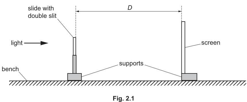
The distance between the slide and the screen is .
The separation of the slits is determined.
Light from a laser is incident normally on the double slit. An interference pattern is observed on the screen. The distance across 10 fringes is measured. The distance between the centres of adjacent fringes is calculated using the equation
The experiment is repeated with slides of different slit separation .
It is suggested that and are related by the equation
where is the wavelength of the incident light.
A graph is plotted of on the -axis against on the -axis.
Determine an expression for the gradient.
gradient = ______
From
So, for a graph of against ,
\lambda D
Background Concept
A straight-line graph has the form
where is the gradient and is the intercept. If the relationship predicts , then a plot through the origin is expected.
Understanding the Question
You are told the relationship for double-slit fringes is
and that a graph is plotted of (vertical axis) against (horizontal axis). The question asks what the gradient of that graph should be in terms of the physical quantities.
Approach
Rearrange the given equation so that is the subject and appears as a factor. Then compare with .
Step-by-Step Reasoning
Start with
Multiply both sides by :
Comparing with shows
Key Takeaways
- To find a gradient expression, rewrite in the form using the graph’s chosen -variable.
Common Mistakes
- Writing (mixing up the rearrangement).
- Treating rather than as the -variable.
Things to Be Careful About
- The gradient carries units: is in mm and in mm, so gradient has units of mm (convert later if needed).
Values of and are given in Table 2.1.
Table 2.1
Calculate and record values of and in Table 2.1. Include the absolute uncertainties in .
Working
For each row:
and for with :
Example (first row):
Answer (Table 2.1 completed)
See completed table in working
Background Concept
When you calculate a new quantity from measured values, you must also propagate the uncertainty.
- For a derived quantity , the calculation is direct.
- For a reciprocal , the uncertainty grows non-linearly as gets smaller.
A standard method for the absolute uncertainty in a reciprocal is:
Understanding the Question
You are given measured slit separations (each with ) and measured distances across 10 fringes. You must fill the missing columns:
- (with absolute uncertainty)
- where
Approach
For each row:
- Compute by dividing by 10.
- Compute .
- Compute the absolute uncertainty in using .
- Round sensibly: uncertainty usually to 1–2 s.f., and the value to the same decimal place.
Step-by-Step Reasoning
Take the first row as a model.
- Calculate the reciprocal:
- Uncertainty in the reciprocal:
- Calculate fringe spacing:
Repeat identically for the other rows.
Key Takeaways
- A reciprocal amplifies uncertainty: smaller gives larger .
- Keep units explicit: in mm gives in mm.
Common Mistakes
- Using (that is for fractional uncertainty, not absolute for the reciprocal).
- Forgetting to include uncertainties in .
- Dividing by 10 but rounding inconsistently.
Things to Be Careful About
- Do not convert some values to metres and others to millimetres in the same table.
- Round the uncertainty to a sensible precision and match the decimal place of the stated value to it.
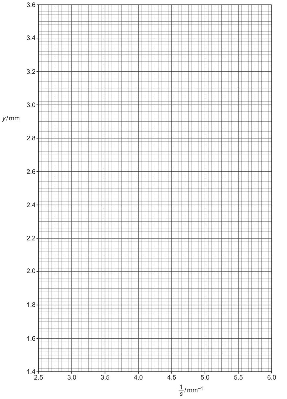
Answer
Plot (vertical) against (horizontal) using the points:
Include horizontal error bars on each point of size :
See graph
Background Concept
For a graph to test a relationship, you must:
- put the correct variable on each axis,
- label axes with quantity and unit,
- choose a sensible scale,
- plot points accurately.
Error bars show the uncertainty range of each point. Here, only has given uncertainties, so the error bars are horizontal.
Understanding the Question
You must plot (calculated from ) against (calculated from ), and you must include error bars for .
Approach
- Use the calculated table values from (b).
- Plot each point where and is fringe spacing.
- Draw an error bar extending left and right from each point by the absolute uncertainty in .
Step-by-Step Reasoning
- Set up axes exactly as required: on vertical, on horizontal.
- Plot all six points.
- For each point, draw a horizontal error bar from to at the same value.
Example: for with , the error bar runs from to .
Key Takeaways
- Horizontal error bars correspond to uncertainty in the -variable.
- Clear axis labels and correct plotting are essential for later gradient determination.
Common Mistakes
- Drawing vertical error bars instead of horizontal ones.
- Plotting instead of .
- Missing units on axes.
Things to Be Careful About
- Use a scale that spreads the points across most of the grid (not cramped into a corner).
- Plot points to at least half a small square accuracy.
Draw the straight line of best fit and a worst acceptable straight line on your graph. Label both lines.
Answer
Draw a straight line of best fit through the plotted points.
Draw a worst acceptable straight line that is still consistent with all the horizontal error bars.
Label the lines clearly as “best fit” and “worst acceptable”.
See graph
Background Concept
A best-fit line represents the overall trend of the data. A worst acceptable line represents an extreme gradient that could still plausibly fit the data given the uncertainties (i.e. it passes through all error bars).
These two lines are used to estimate uncertainty in the gradient:
- best-fit gives the central value,
- worst acceptable gives an extreme allowed value.
Understanding the Question
You have already plotted against and included horizontal error bars. Now you must add:
- a best-fit straight line,
- a worst acceptable straight line,
and label both.
Approach
- Best-fit: balance the line so roughly equal scatter above and below.
- Worst acceptable: make the gradient as steep or as shallow as possible while still crossing every point’s uncertainty range (every horizontal error bar).
Step-by-Step Reasoning
- Place a ruler and adjust until the line represents the trend (do not join dot-to-dot).
- For worst acceptable: pivot the ruler about one end so the line becomes as steep/shallow as possible but still intersects every horizontal error bar.
- Write labels next to each line so the examiner can identify them.
Key Takeaways
- Worst acceptable line must be consistent with uncertainties, not just the plotted central points.
- Labeling matters: the examiner must know which line is which.
Common Mistakes
- Drawing a second random line that does not pass through all error bars.
- Forgetting to label the lines.
- Forcing the line through every central point (not required and usually impossible).
Things to Be Careful About
- If the relationship predicts a line through the origin, your best-fit line should be close to the origin, but you should still follow the plotted data and error bars.
- Worst acceptable line must still be straight (use a ruler).
Determine the gradient of the line of best fit. Include the absolute uncertainty in your answer.
gradient = ______
Working
Using the line of best fit, take two well-separated points on the line (example readings):
From the worst acceptable line, take its gradient and find
Answer
(0.60 \u00b1 0.02) mm^2
Background Concept
The gradient of a straight-line graph is
To reduce percentage reading error, you should use a large triangle on the line (choose points far apart). For uncertainty in gradient, Paper 5 commonly uses:
where is the gradient of a worst acceptable straight line consistent with the error bars.
Understanding the Question
You have drawn two lines on the same vs graph:
- best-fit line,
- worst acceptable line.
You must calculate the best-fit gradient and an absolute uncertainty based on how different the worst acceptable gradient is.
Approach
- Read two widely separated points on the best-fit line (not necessarily on plotted data points).
- Compute .
- Repeat for the worst acceptable line to get .
- Use .
Step-by-Step Reasoning
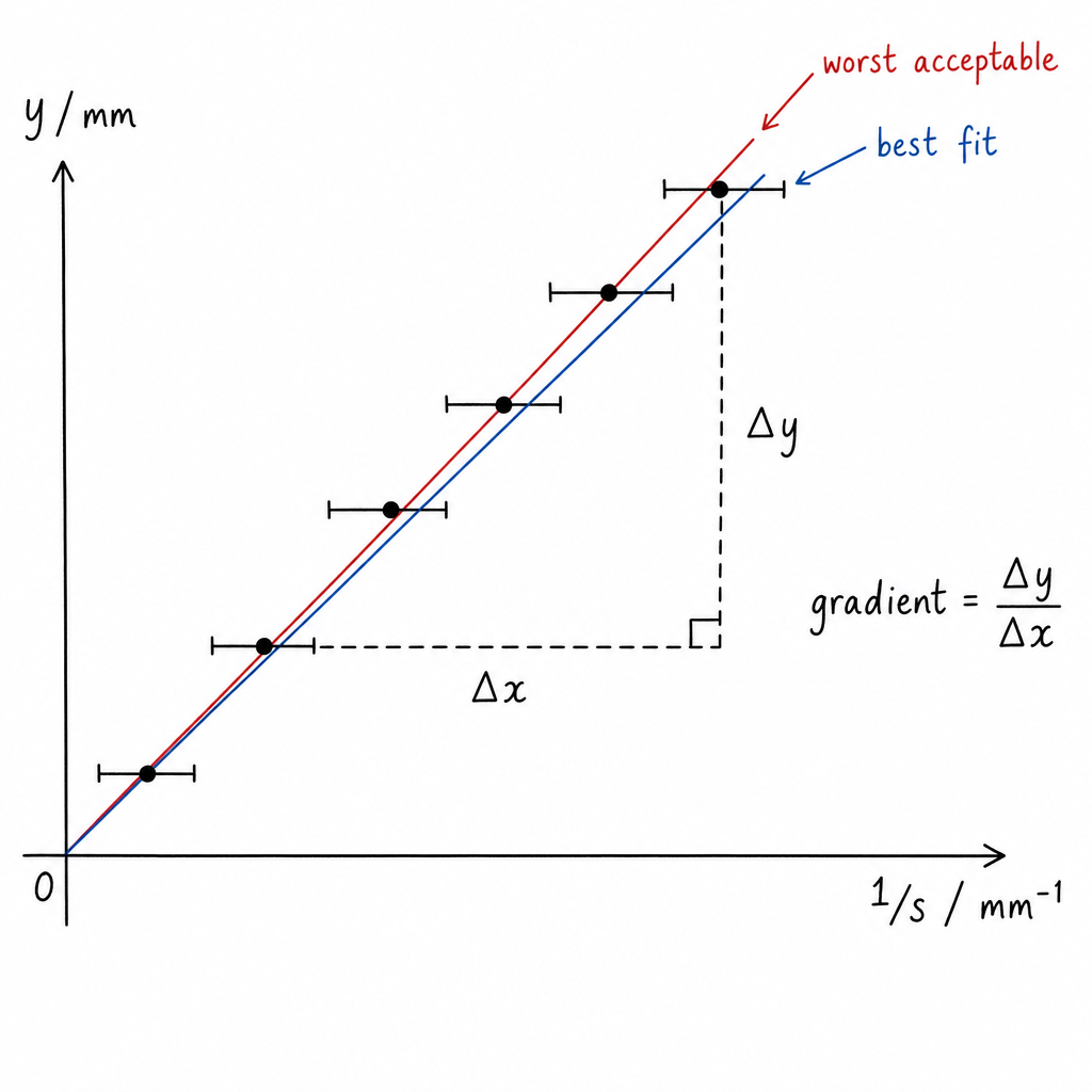
- Pick two points on the best-fit line with a large horizontal separation.
- Calculate the differences:
-
Divide to get the gradient and include units:
- is in mm,
- is in mm,
- so gradient units are mm.
-
For the uncertainty, repeat the gradient calculation for the worst acceptable line.
-
The absolute uncertainty is the difference between the two gradients.
Key Takeaways
- Use a large triangle to improve accuracy.
- Worst acceptable line + best-fit line is the standard method for gradient uncertainty in Paper 5.
Common Mistakes
- Using two adjacent grid points (tiny triangle) leading to large rounding error.
- Calculating instead of .
- Using two data points instead of two points on the best-fit line.
- Quoting uncertainty as a percentage when the question asks for absolute uncertainty.
Things to Be Careful About
- Make sure you use the same units as the axes when calculating the gradient.
- Round the uncertainty sensibly (usually 1 s.f. or 2 s.f.) and match the main value to that precision.
The distance between the slide and the screen is measured several times:
Determine the mean distance . Include the absolute uncertainty.
= ______
Working
Mean distance:
Uncertainty (half-range):
Answer
(0.921 \u00b1 0.008) m
Background Concept
When a quantity is measured repeatedly, the best estimate is usually the mean. A simple estimate of the absolute uncertainty from repeats is half the range:
This reflects the spread of the readings.
Understanding the Question
You are given five measurements of the distance between the double slit and the screen. You must find:
- the mean ,
- an absolute uncertainty.
Approach
- Add all five values and divide by 5 to get .
- Find the maximum and minimum readings.
- Compute as half the range.
Step-by-Step Reasoning
- Mean:
- Range method:
So report with the uncertainty.
Key Takeaways
- Mean gives the best central value; half-range gives a quick uncertainty estimate.
Common Mistakes
- Using the full range instead of half the range.
- Quoting too many decimal places compared with the uncertainty.
Things to Be Careful About
- Keep units as metres throughout.
- Make the number of decimal places in consistent with the uncertainty (here to is fine).
Using your answers to (a), (c)(iii) and (d), determine the value of . Include an appropriate unit.
= ______
Working
From (a),
Convert gradient to SI:
Using :
Answer
6.5 \u00d7 10^-7 m
Background Concept
From double-slit interference geometry, the fringe spacing is inversely proportional to slit separation :
So the gradient of a graph of vs is . This allows to be found from experimental data.
Understanding the Question
You already determined:
- expression for gradient: ,
- numerical gradient from the graph,
- mean distance .
Now you must find the wavelength with a suitable unit.
Approach
- Rearrange: .
- Ensure units are consistent (convert mm to m).
- Substitute values.
Step-by-Step Reasoning
- Rearrangement:
- Unit conversion is essential because is in metres. If the gradient was read in mm:
So multiply the mm value by to get m.
- Substitute into to get in metres.
Key Takeaways
- The slope of a carefully chosen linear graph can directly give physical constants.
- Always check and convert units before calculating constants.
Common Mistakes
- Forgetting to convert mm to m (gives wavelength wrong by ).
- Using (inverting incorrectly).
Things to Be Careful About
- Quote the final wavelength to a sensible number of significant figures, consistent with the gradient and values.
- Use SI unit (or nm if explicitly converted and stated).
Working
Since
Answer
4.2 %
Background Concept
For multiplication/division, fractional (or percentage) uncertainties add:
If
then
This is the standard A-Level rule used for experimental uncertainties.
Understanding the Question
You found using
You also have absolute uncertainties in the gradient and in . You must combine them to get the percentage uncertainty in .
Approach
- Convert each absolute uncertainty into a fractional uncertainty.
- Add the fractional uncertainties (because it is a division).
- Multiply by 100 to get a percentage.
Step-by-Step Reasoning
- Fractional uncertainty in gradient:
- Fractional uncertainty in :
- Add them to get and multiply by .
Key Takeaways
- For , uncertainties in and both contribute.
- Percentage uncertainty is often dominated by the quantity with the larger fractional uncertainty (here, the gradient).
Common Mistakes
- Subtracting uncertainties because it is a division (they still add as fractions).
- Using absolute uncertainties directly without dividing by the measured value first.
Things to Be Careful About
- Use consistent significant figures: a final percentage uncertainty is usually quoted to 1 d.p. or 2 s.f.
- Ensure you use the same and values as in part (c)(iii).
The experiment is repeated. Determine the slit separation that gives a value of of . Include the absolute uncertainty.
= ______
Working
Given :
Using
With and :
Uncertainty:
Answer
(1.20 \u00b1 0.07) \u00d7 10^-4 m
Background Concept
The double-slit formula links slit separation , fringe spacing , screen distance , and wavelength :
If you want a particular fringe spacing , you can rearrange to find the required slit separation:
Uncertainty propagation for multiplication/division uses fractional uncertainties:
Understanding the Question
A repeat of the experiment aims for a fringe spacing of with uncertainty . Using your measured wavelength (and the screen distance), you must calculate the slit separation that would produce this spacing, and give its absolute uncertainty.
Approach
- Convert from cm to m (including its uncertainty).
- Rearrange to .
- Calculate .
- Find percentage uncertainty in by adding the percentage uncertainties from , , and .
- Convert back to an absolute uncertainty: .
Step-by-Step Reasoning
- Convert:
and
- Rearrange and substitute into
-
For uncertainty:
- if has percentage uncertainty from part (e)(ii), use that directly,
- add ,
- add .
-
Convert total percentage uncertainty into absolute uncertainty in .
Key Takeaways
- Smaller gives larger (since ).
- Always convert cm to m before using equations that expect SI units.
- For products/quotients, add percentage uncertainties.
Common Mistakes
- Using (incorrect rearrangement).
- Forgetting to convert to metres.
- Ignoring the uncertainty in .
Things to Be Careful About
- Keep the uncertainty to 1–2 significant figures and match the main value’s precision.
- Be consistent about whether you are using from (d) and from (e), and include the corresponding uncertainties.