Physics 9702/53 — October/November 2025
Cambridge A-Level · Planning, Analysis and Evaluation · worked solutions for every part, with the mark scheme
Topics Analysis, Conclusions and Evaluation · Planning
On a bench, a steel ball of radius is used to compress a spring by a distance . The ball is held at rest in this position, as shown in Fig. 1.1.
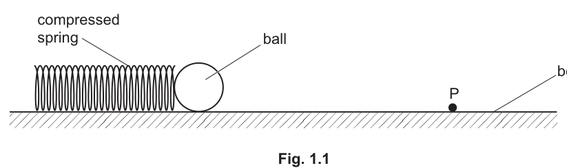
The ball is released and rolls along the bench. At a fixed point P, the ball has speed . The speed of the ball at P is determined using one light gate connected to a timer.
Several steel balls of different radii are available.
It is suggested that is related to by the relationship
where is the spring constant of the spring, is the density of the steel, and and are constants.
Plan a laboratory experiment to test the relationship between and .
Draw a diagram showing the arrangement of your equipment.
Explain how the results could be used to determine values for and .
In your plan you should include:
• the procedure to be followed
• the measurements to be taken
• the control of variables
• the analysis of the data
• any safety precautions to be taken.
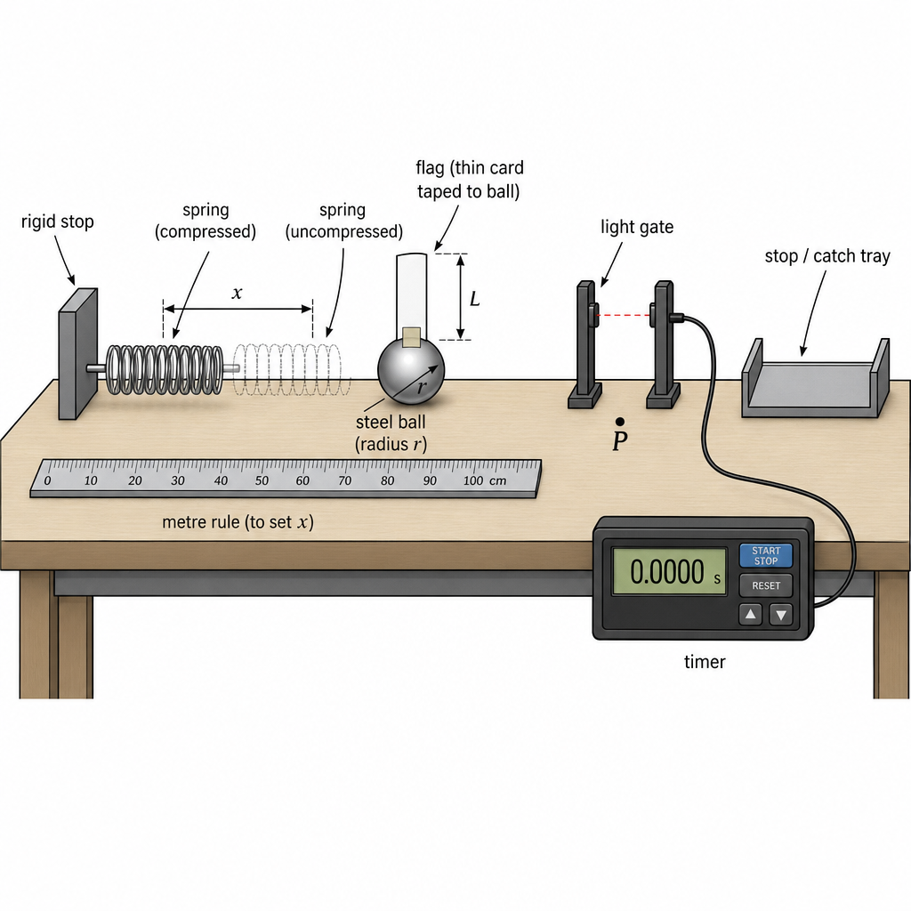
Variables
- Independent variable: ball radius (use different steel balls).
- Dependent variable: speed of the ball at fixed point .
- Controlled variables: spring compression , same spring (same ), same position of (same distance from release point), same bench surface/track and alignment, same light-gate/flag arrangement.
Apparatus
Spring and rigid stop, clamp stand, metre rule/set square, set of steel balls, vernier callipers/micrometer, light gate + timer, thin card “flag” of known length (same for all trials) taped to ball, tape measure to locate , tray/stop to catch ball.
Procedure and measurements
- Determine for the spring (if not given): hang known masses, measure extension, plot against extension; gradient .
- Mark point at a fixed distance from the release position.
- Fix the light gate at and connect to timer (mode: measure time beam is interrupted).
- Attach the same light flag of length to each ball; measure with callipers.
- For a chosen ball, measure its diameter with callipers and calculate .
- Compress the spring by a fixed distance using a metre rule (measure from uncompressed position). Hold the ball at rest against the spring, then release without pushing.
- Record the interrupt time when the flag passes the light gate.
- Repeat at least 3 times for the same ball and take mean .
- Repeat steps 5–8 for at least 6 balls of different radii.
Calculations
For each ball:
Analysis (to determine and )
Given
Take logs:
Plot (y-axis) against (x-axis).
- Gradient .
- Intercept , so
A straight line supports the suggested relationship.
Control of variables
- Use the same spring throughout and keep constant.
- Keep fixed and do not move the light gate between runs.
- Use the same flag length and same release method.
- Keep bench/track clean and level; ensure ball rolls along the same line.
Safety
- Keep face/hands away from the spring and ball line of motion during release.
- Use a stop/tray to prevent the ball falling off the bench.
- Ensure clamp stand/light gate is stable to avoid toppling.
See working
Background Concept
The suggested relationship is
This has the structure of a power law in : keeping , and constant, it predicts
To test a power law experimentally, we typically:
- measure for different values of while holding other variables constant, and
- transform the equation into a straight-line form so that a graph’s gradient and intercept give the constants.
A single light gate measures the time for an object (or a fixed “flag” attached to it) to block the beam. If the blocked length is known (call it ), the instantaneous speed at the gate is
Understanding the Question
You have steel balls of different radii . Each ball is launched by a spring compressed by a fixed distance , and you need the speed at a fixed point . You are constrained to using one light gate and a timer.
You must produce a workable plan including: apparatus/diagram, procedure, measurements, controls, data analysis, and safety. You must also explain how to obtain both constants and from the results.
Approach
- Choose as the independent variable (use different balls).
- Measure at point using one light gate by attaching a flag of known length to the ball; record interrupt time and compute .
- Keep constant and keep everything else (spring, surface, point , light-gate setup) constant so that any change in is due to changing .
- Linearise the model with logarithms:
so a plot of vs is a straight line with gradient . The intercept gives .
Step-by-Step Reasoning
1) Measuring the radii
For each ball, measure the diameter with vernier callipers or a micrometer (take several readings at different orientations and average to reduce random error). Then
2) Keeping the launch conditions constant
- Use the same spring for all trials (so is constant).
- Set the compression to the same value each time using a ruler fixed alongside the spring.
- Release the ball from rest without giving it an extra push (e.g. hold with a card/trigger and pull it away cleanly).
- Keep the point fixed (mark it on the bench) and keep the light gate fixed at .
3) Using one light gate to obtain speed at P
A single light gate gives a time interval for which the beam is interrupted. To turn this into a speed, you must know the length that passes through the beam during that time.
A common robust method is:
- Attach a thin card “flag” of known length to the ball (keep the same flag for all balls, or make identical flags).
- Measure with callipers.
- When the ball passes through the gate, the timer reads the interrupt time .
Then compute
Repeat at least 3 times for each ball and average (or average ) to reduce random uncertainty.
4) Processing and linearising the data
From the suggested equation,
take base-10 logs (natural logs also fine if used consistently):
This matches the straight-line form if we set:
- ,
- ,
- gradient ,
- intercept .
So:
- Find from the gradient: .
- Find from the intercept:
If the plotted points lie close to a straight line (within experimental scatter), that supports the proposed relationship.
5) Control of variables (what to state explicitly)
Creditworthy controls are those that directly affect energy transfer and energy losses:
- Compression : keep fixed, because the model predicts .
- Same spring: keeps constant.
- Same point and same gate position: ensures the same distance travelled before measuring (so losses are comparable).
- Same surface/track and alignment: frictional losses change ; keep the bench level and clean.
- Same flag length and same gate mode: ensures the speed calculation method does not change between balls.
6) Safety
Main hazards are the spring release and the ball rolling/falling:
- Keep hands/face away from line of motion; do not lean over the spring on release.
- Use a catch tray/stop at the end of the bench.
- Clamp equipment securely so the gate/stand cannot topple.
Key Takeaways
- A single light gate measures a time interval; you need a known interrupt length to convert that into speed.
- Testing a power law is best done by log-linearising and plotting a straight-line graph.
- Gradient gives the exponent (), intercept gives the constant () once other parameters are known/controlled.
- A strong plan always identifies variables, controls, repeats, and a clear graph-based method for determining constants.
Common Mistakes
- Not stating how is obtained from one light gate (you must include a measured length such as a flag length).
- Changing more than one variable at a time (e.g. varying as well as ).
- Plotting against without linearising, which makes extracting and unreliable.
- Forgetting that the graph gradient gives (sign error).
- Not including repeats/averaging for each radius.
Things to Be Careful About
- Ensure the flag is rigidly attached and does not flap; otherwise the interrupt time is inconsistent.
- Measure carefully (callipers perpendicular to diameter; repeat and average).
- Keep the light gate aligned so the flag cleanly blocks the beam each time.
- When using logs, be consistent about base (10 or ) and use the matching inverse when finding .
- If you determine yourself, take enough data points and use a best-fit line for vs extension to reduce uncertainty.
A student investigates light from different galaxies.
Fig. 2.1 shows the lines in the absorption spectrum from a distant galaxy.
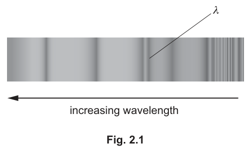
The wavelength of one of the lines in the absorption spectrum is . The wavelength of this spectral line in the laboratory is .
The observations of the same spectral line are repeated for different galaxies.
The student determines the distance of each galaxy from the Earth.
It is suggested that and are related by the equation
where is the speed of light in free space and is the Hubble constant.
A graph is plotted of on the -axis against on the -axis.
Determine expressions for the gradient and -intercept.
gradient = ______
-intercept = ______
Working
From
Answer
gradient
-intercept
gradient = (\lambda_0H), y-intercept = (\lambda_0)
Background Concept
To analyse experimental data, we often rearrange an equation into the straight-line form
where:
- is the gradient (slope) of the graph,
- is the -intercept (value of when ).
If you plot the correct variables on the axes, you can extract physical constants from and .
Understanding the Question
You are given the relationship
and you are told the student plots a graph of (vertical axis) against (horizontal axis). You must rewrite the equation so that it looks like .
Approach
- Multiply both sides by to remove the fraction.
- Make the subject.
- Compare directly with where and .
Step-by-Step Reasoning
Start with
Multiply by :
Add to both sides:
Rewrite to show as a factor:
So on a graph of (as ) against (as ):
- gradient
- intercept .
Key Takeaways
- Always convert the physics equation to using the actual plotted axes.
- The intercept is the value of at .
Common Mistakes
- Leaving the equation in terms of (that would correspond to plotting a different variable).
- Giving gradient as or similar due to incorrect algebra.
Things to Be Careful About
- The graph is vs (not vs ), so you must isolate .
- Keep track of brackets: the gradient is the entire coefficient multiplying , i.e. .
Values of and are given in Table 2.1.
Table 2.1
The value of is .
Calculate and record values of in Table 2.1. Include the absolute uncertainties in .
Working
Uncertainty:
Values (in units of ):
- :
- :
- :
- :
- :
- :
Answer
:
, , , , ,
1.60±0.40, 3.47±0.40, 4.83±0.40, 6.00±0.40, 9.50±0.40, 12.5±0.40 (all in units of 10^15 s)
Background Concept
When you create a new column in a data table using a formula, you must:
- Calculate the derived quantity.
- Propagate uncertainties correctly.
Here,
is obtained by dividing the distance by the speed .
For multiplication/division by a constant, the absolute uncertainty scales by the same factor:
Understanding the Question
The table gives in units of with an absolute uncertainty for every row. You must calculate (in seconds) and record it in the table as
and include the absolute uncertainty in .
Approach
- Convert each distance into a time using .
- Because is fixed and exact for this calculation, divide both the central value and the absolute uncertainty in by .
- Finally, express the result in units of to match the table.
Step-by-Step Reasoning
Given
For any row,
Example (first row):
Uncertainty in (same method for all rows because is the same each time):
So each table entry becomes “value ” in the table’s unit of .
Key Takeaways
- Dividing by a constant divides the absolute uncertainty by the same constant.
- Match the powers of ten and units used in the table heading.
Common Mistakes
- Forgetting to include the uncertainty in .
- Putting percentage uncertainty instead of absolute uncertainty.
- Forgetting the table’s scaling () and writing the raw seconds value.
Things to Be Careful About
- Keep the uncertainty to an appropriate number of significant figures (typically 1 or 2), and match the decimal places of the value to the uncertainty.
- Use (not ) because is in km.
Answer
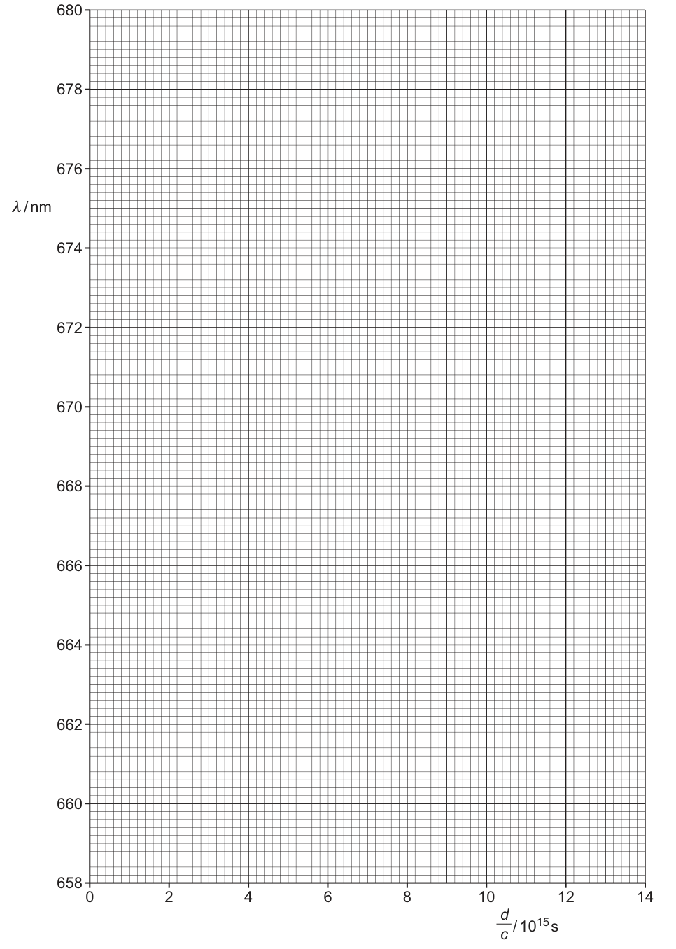
Plot the points with and :
, , , , , .
Add horizontal error bars of on each -value.
See graph (points plotted with ±0.40 horizontal error bars).
Background Concept
A graph is used to test whether two quantities are linearly related. Good graph technique (Paper 5) includes:
- Correct axes with quantity and unit.
- A sensible scale using at least half the grid.
- Accurate plotting (fine pencil, small crosses/dots).
- Error bars representing absolute uncertainty in the measured quantity.
Here, the uncertainty is in , so you add horizontal error bars.
Understanding the Question
You must plot (in nm) on the -axis against on the -axis using the values you calculated in part (b). You must include error bars for using the absolute uncertainties you found.
Approach
- Label axes exactly as requested.
- Choose scales that spread the data well across the grid.
- Plot each point accurately.
- For each point, draw a horizontal line segment representing where .
Step-by-Step Reasoning
- Your values range roughly from to , so the given 0 to 14 scale is appropriate.
- Your values range from about to , so the given 658 to 680 scale is appropriate.
For each data point:
- Plot a small cross at .
- Draw the horizontal error bar from to .
Example: for , draw the bar from to at .
Key Takeaways
- Error bars go on the axis of the quantity that has uncertainty.
- Error bars are drawn using absolute uncertainty, not percentage uncertainty.
Common Mistakes
- Drawing vertical error bars (there is no uncertainty given for ).
- Using the uncertainty in instead of the uncertainty in .
- Plotting with poor scale so the points are bunched into a corner.
Things to Be Careful About
- Ensure the error bar half-length is exactly in the graph’s units.
- Do not join the points dot-to-dot; the line is drawn in part (ii).
Draw the straight line of best fit and a worst acceptable straight line on your graph. Label both lines.
Answer
Draw a single straight line of best fit (balanced about the plotted points).
Draw a worst acceptable straight line (steepest or shallowest) that still passes through all the horizontal error bars.
Label both lines clearly (e.g. “best fit” and “worst acceptable”).
See graph (best-fit line and labelled worst acceptable line).
Background Concept
A line of best fit represents the overall linear trend of the data. In Paper 5, uncertainties in gradient and intercept are often estimated using a worst acceptable line:
- Draw the best-fit line first.
- Then draw the steepest (or shallowest) straight line that is still consistent with the error bars of all points.
- The difference between the gradients (or intercepts) of these two lines gives an estimate of the uncertainty.
Understanding the Question
You already plotted vs with horizontal error bars. Now you must:
- Draw the best-fit straight line.
- Draw a worst acceptable straight line.
- Label both.
Approach
- Best-fit line: place it so that points are roughly equally scattered above and below, not forced through every point.
- Worst line: choose either the steepest or shallowest line that still intersects every point’s error bar region.
Step-by-Step Reasoning
- Using a ruler, draw the straight line that best represents the trend. It should go through the “middle” of the error-bar rectangles and not be kinked.
- Now try to rotate the line to make it as steep as possible while still crossing each horizontal error bar (i.e. for each point at height , the line’s value at that must lie within ).
- If making it steeper fails to pass through one point’s error bar, reduce steepness until it just fits.
- If the steepest line is very close to the best fit, try the shallowest line instead; you will use whichever gives the larger difference from best fit.
Key Takeaways
- Best fit is about overall trend; worst line is about extremal gradient still allowed by the uncertainties.
Common Mistakes
- Drawing the worst line without checking it intersects all error bars.
- Drawing two worst lines but not clearly identifying which is used later.
- Forcing the best-fit line through the origin (not justified here).
Things to Be Careful About
- Use a ruler; freehand lines typically lose the mark.
- Label the lines directly on the graph so the examiner can tell which is which.
Determine the gradient of the line of best fit. Include the absolute uncertainty in your answer.
gradient = ______
Working
Using two well-separated points on the best-fit line (example): and ,
Worst acceptable gradient (from worst line): (or ).
Answer
(1.83 ± 0.14) nm per (10^15 s)
Background Concept
For a straight-line graph against , the gradient is
To reduce percentage error, you must use a large triangle: pick two points far apart on the line, not necessarily the original plotted points.
To estimate uncertainty in gradient on a graph with error bars:
- find from the best-fit line;
- find from the worst acceptable line;
- take
Understanding the Question
You must read the gradient of the line of best fit from your graph of vs , and include an absolute uncertainty obtained from the difference between best and worst acceptable lines.
Approach
- Choose two widely separated points on the best-fit line, read and .
- Compute .
- Repeat using the worst acceptable line to get .
- Use .
Step-by-Step Reasoning
- Suppose two points on the best-fit line are read as and .
Compute:
So
Then from the worst acceptable line you might obtain, for example, (or a steepest line giving ). The uncertainty is the larger difference from :
Hence in the graph’s units.
Key Takeaways
- Always use two points far apart on the drawn line.
- Uncertainty comes from comparing best-fit and worst acceptable gradients.
Common Mistakes
- Using two nearby points, giving a large percentage uncertainty.
- Using instead of .
- Calculating uncertainty as half the difference without being instructed; Paper 5 typically uses the full difference between best and worst.
Things to Be Careful About
- Make sure uses the graph’s units (here ).
- Read points from the line, not from the data table.
Determine the -intercept of the line of best fit. Include the absolute uncertainty in your answer.
-intercept = ______
Working
From the best-fit line, at :
From the worst acceptable line, intercept .
Answer
(655.1 ± 1.3) nm
Background Concept
For a straight-line graph , the -intercept is the value of when .
Graphically, it is where the drawn line crosses the -axis.
Uncertainty in the intercept is estimated similarly to the gradient:
Understanding the Question
You must read the -intercept of the best-fit line on your vs graph, and estimate its absolute uncertainty using the worst acceptable line.
Approach
- Extend the best-fit line to the -axis (at ) and read .
- Extend the worst acceptable line to the -axis and read .
- Take .
Step-by-Step Reasoning
- On the best-fit line, at the intercept is read as about .
- On the worst acceptable line, the intercept might be read as about .
So the absolute uncertainty estimate is
Hence
Key Takeaways
- The intercept is the physical value of at zero .
- Use best vs worst acceptable line to estimate its uncertainty.
Common Mistakes
- Reading the intercept from the data table rather than from the drawn line.
- Forgetting to extend the line to (especially if it doesn’t naturally reach the axis on the drawn segment).
Things to Be Careful About
- Read the intercept to the resolution allowed by the graph scale.
- Keep the uncertainty consistent with the precision of the intercept reading.
Using your answers to (a), (c)(iii) and (c)(iv), determine the values of and . Include appropriate units.
= ______
= ______
Working
From (a):
- -intercept
- gradient
From (c)(iv):
Graph uses , so
Hence
With and :
Answer
λ0 = 655 nm, H = 2.8 × 10^-18 s^-1
Background Concept
When you have a best-fit line for a linearised relation, you can map the graph equation onto the physics equation.
From part (a) we found
So:
- intercept
- gradient (with respect to measured in seconds) .
However, if the plotted axis is scaled (here ), the graph gradient is also scaled.
Understanding the Question
You have measured from the graph:
- best-fit gradient (in nm per unit of )
- best-fit intercept (in nm)
You must use these to calculate and the Hubble constant with units.
Approach
- Set equal to the -intercept.
- Correctly interpret the gradient with the axis scaling: if , then .
- Substitute into the linear equation and match coefficients to extract .
Step-by-Step Reasoning
From (a):
But the graph uses
Substitute into the equation:
So the gradient on the plotted graph is
Therefore
Using representative best-fit results and :
The intercept gives
Key Takeaways
- Intercept directly gives .
- Gradient gives only after accounting for the axis scaling factor ( here).
Common Mistakes
- Using and forgetting the scale factor.
- Giving in the wrong units (it should be ).
Things to Be Careful About
- The units cancel for nm in , leaving as required.
- Use consistent significant figures (typically 2 s.f. for from a graph).
Hubble’s law suggests that the age of the universe is related to by
Determine a value for . Include the absolute uncertainty in your answer.
= ______
Working
Using ,
For , fractional uncertainty:
Answer
(3.6 ± 0.3) × 10^17 s
Background Concept
If a quantity is calculated from a measured value, you must propagate the uncertainty.
For a reciprocal relationship
the fractional (percentage) uncertainty in equals the fractional uncertainty in :
Then the absolute uncertainty is
Understanding the Question
You have found from the graph and must use
to estimate the age of the universe in seconds, including an absolute uncertainty.
Approach
- Calculate using .
- Use the rule for powers: for , the fractional uncertainty in equals that in .
- Convert back to an absolute uncertainty in seconds.
Step-by-Step Reasoning
Using a representative value from part (d), e.g.
calculate :
Fractional uncertainty in :
So fractional uncertainty in is the same:
Hence
So
Key Takeaways
- For , the fractional uncertainty transfers directly from to .
- Quote uncertainty to 1 significant figure (or 2 if it begins with 1 or 2), and match the value’s precision accordingly.
Common Mistakes
- Using absolute uncertainty directly (e.g. ), which is not valid.
- Forgetting that the uncertainty should be absolute in seconds, not a percentage.
- Rounding too aggressively compared with .
Things to Be Careful About
- Keep powers of ten consistent: .
- If your value of differs slightly (because it depends on your graph), your will differ; the method of uncertainty propagation is what is being assessed.