Physics 9702/52 — October/November 2025
Cambridge A-Level · Planning, Analysis and Evaluation · worked solutions for every part, with the mark scheme
Topics Analysis, Conclusions and Evaluation · Planning
Fig. 1.1 shows a model wind turbine with blades, each of length , placed in moving air.
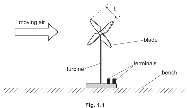
The area of the circle swept by the blades of the turbine is .
The output of the turbine has two terminals. The turbine is connected to a resistor of resistance . At a speed of the moving air, the current in the resistor is .
The atmospheric pressure is and the thermodynamic temperature of the air is .
It is suggested that is related to by the relationship
where is a constant.
Plan a laboratory experiment to test the relationship between and .
Draw a diagram showing the arrangement of your equipment.
Explain how the results could be used to determine a value for .
In your plan you should include:
- the procedure to be followed
- the measurements to be taken
- the control of variables
- the analysis of the data
- any safety precautions to be taken.
Variables
- Independent variable: air speed .
- Dependent variable: current in the load resistor.
- Controlled: load resistance ; blade length (hence swept area ); turbine position/orientation relative to airflow; air temperature ; atmospheric pressure (as constant as possible during the run).
Apparatus
Model wind turbine, variable-speed fan / wind tunnel, anemometer, fixed resistor (suitable power rating), ammeter (or data logger), switch, connecting leads, thermometer, barometer (or obtain local atmospheric pressure), metre rule/vernier calipers, clamp stand.
Diagram
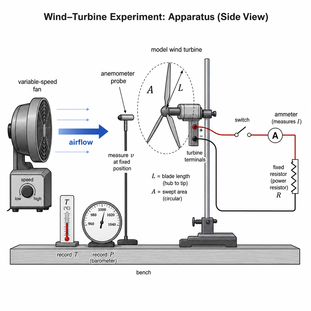
Procedure and measurements
- Measure blade length and calculate .
- Set up the turbine a fixed distance from the fan (or in a wind tunnel) and clamp securely.
- Connect the turbine terminals to the fixed resistor in series with an ammeter.
- Place the anemometer at a fixed position near the turbine (e.g. just upstream of the rotor) and keep this position the same for all readings.
- Set a fan speed, allow readings to stabilise, then record and the steady current .
- Repeat for at least 6 different values of over a wide range. Repeat each reading and average and .
- Measure/record air temperature during the experiment and atmospheric pressure .
Analysis of data
Compute for each run:
and
Plot a graph of (y-axis) against (x-axis).
Determination of
From
rearrange to
So the graph of against should be a straight line through the origin with gradient
Hence
(using measured , and recorded and ).
Safety
- Keep hands/hair clear of rotating blades; use a guard/goggles.
- Clamp turbine and fan securely to prevent movement.
- Use a resistor with adequate power rating; switch off between readings to avoid overheating.
See working
Background Concept
The suggested relationship is
Here is the current in a resistor of resistance , so is the electrical power dissipated in the resistor (because ). The right-hand side depends on the air speed (as ) and on properties/conditions of the air ( and ) and the turbine swept area .
To “test the relationship” you should vary one quantity (here ) and measure the responding quantity (), while keeping the other variables constant or measuring them so they can be accounted for. You then check whether the data are consistent with the predicted functional form (here a straight-line relationship between and ).
A common Paper 5 method is to rearrange the given equation into the linear form
and then use a graph to obtain the gradient and hence determine the unknown constant (here ).
Understanding the Question
You are given a model wind turbine connected to a resistor . When air of speed blows on it, a current flows in the resistor.
You must plan an experiment that:
- changes in a controlled way,
- measures for each ,
- keeps , and the set-up geometry fixed,
- measures (or keeps constant) and ,
- uses an appropriate graph to decide whether the proposed relationship is correct,
- shows how to extract a value of from your results.
Because this is a planning question, credit comes from: a workable set-up, correct identification of variables, enough readings and repeats, and a clear linearisation/graph leading to .
Approach
- Choose a way to produce controllable airflow: a variable-speed fan at a fixed distance, or a wind tunnel.
- Measure air speed with an anemometer at a fixed position relative to the turbine.
- Connect the turbine to a known fixed resistor and measure current with an ammeter/data logger.
- Take many pairs of readings over a wide range, with repeats.
- Linearise the equation by rearranging to the form where the constant contains .
- Plot against ; if the model is correct you should get a straight line through the origin.
- Use the gradient and the measured/recorded values of , and to calculate .
Step-by-Step Reasoning
1) Set-up and measurements
You need both an electrical measurement and an airflow measurement.
- Electrical side: connect the turbine terminals to a fixed resistor (so is controlled) and place an ammeter in series to measure . A data logger can improve resolution and allow you to average a steady reading.
- Air speed: put an anemometer just upstream of the turbine rotor. The key is consistency: the measured speed must correspond to the air that actually reaches the blades.
Measure blade length using a ruler/vernier. The swept area is the area of the circle traced out by the blade tips:
2) Control of variables
- : use the same resistor throughout; do not change it between runs.
- Geometry: keep the turbine at the same distance from the fan and aligned with the airflow; clamp it so it cannot rotate away.
- : do not change blade length/pitch during the experiment.
- and : in a school lab these do not change much during one session; still, you should measure with a thermometer and obtain from a barometer (or a nearby weather station reading). Record them and use the average values in the calculation of .
3) Taking enough data
For a relationship test, you need a range of values and multiple repeats:
- Choose at least 6 different fan settings (or wind tunnel speeds) covering a wide range of .
- For each , wait until the speed and current stabilise, record and , then repeat and average.
Repeats reduce random uncertainty, especially because both and can fluctuate.
4) Linearising and graphing
Start from
Multiply both sides by :
This has the linear form with:
- gradient
So you calculate and for each run and plot (y-axis) against (x-axis). A straight line close to the origin supports the suggested model.
5) Extracting
From the gradient expression,
rearrange to obtain
So once the best-fit gradient is found from the graph, you substitute:
- (in kelvin),
- (in pascal),
- (in ),
- and the measured gradient .
If you include uncertainty work, a good method is to draw a worst acceptable line to estimate uncertainty in , then propagate that to .
6) Safety
Main hazards:
- rotating blades (impact/cuts) and flying debris,
- unstable equipment due to airflow,
- resistor heating (burn risk).
Controls:
- keep hands/hair away, consider a guard and eye protection,
- clamp turbine and fan securely,
- use a suitably rated resistor and switch off between readings.
Key Takeaways
- In planning questions, define independent/dependent/controlled variables clearly.
- Make the experiment repeatable: fixed geometry, consistent sensor placement, multiple readings.
- Linearise the given equation to decide what graph gives a straight line.
- Use the gradient of the straight line to determine the constant ( here).
Common Mistakes
- Plotting against directly (will not be linear if the model is ).
- Forgetting to keep constant or not stating how is controlled.
- Measuring at different positions for different runs (changes the effective speed).
- Not including how to obtain (must use from measuring ).
- Not stating that you need multiple values of and repeats.
Things to Be Careful About
- Units: use SI units ( in , in , in , in ).
- The graph should be vs (or equivalently vs if is constant, but then include correctly when finding ).
- Ensure the best-fit line is judged properly; if it does not pass near the origin, that suggests systematic error (e.g. background current offset or incorrect speed measurement).
- Resistor temperature rise can change ; mitigate by using a high power resistor and brief measurement times (or measure before/after).
A student observes the orbits of some of the moons around the planet Saturn, as shown in Fig. 2.1.
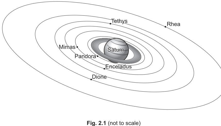
For the moon Pandora, the period of the orbit and the mean distance from the centre of Saturn are determined.
The measurements of period and mean distance are repeated for other moons.
It is suggested that and are related by the equation
where and are constants.
A graph is plotted of on the -axis against on the -axis.
Determine expressions for the gradient and -intercept.
gradient = ______
-intercept = ______
Let
From
Also and , so
Therefore
gradient
-intercept
gradient = n; y-intercept = lg(2π/k) + 8n − 3
Background Concept
A relationship of the form
is a power law in . A standard way to test a power law with experimental data is to take common logarithms (), because powers turn into multiplication:
A graph of against should therefore be a straight line, and the exponent becomes the gradient.
Understanding the Question
You are told that a graph is plotted with
- -axis: (but actually is used later),
- -axis: (later written as ).
You must rearrange the given equation into the straight-line form , so you can state expressions for the gradient and intercept .
Approach
- Take of both sides of .
- Replace and by the plotted quantities, which are scaled by powers of 10.
- Compare with .
Step-by-Step Reasoning
Start with
Take :
Now define what is actually plotted:
so .
Similarly,
so .
Substitute into the logged equation:
and rearrange:
So the gradient is and the intercept is the bracketed constant.
Key Takeaways
- Taking logarithms turns a power law into a straight line.
- Axis scalings like and shift the intercept but do not change the gradient.
Common Mistakes
- Forgetting that and .
- Writing the intercept as just (missing the extra ).
Things to Be Careful About
- The gradient is unchanged by multiplying/dividing by powers of 10; only the intercept shifts.
- Make sure you use common log (), not natural log (), since the axes are labelled .
Values of and are given for different moons in Table 2.1.
Table 2.1
| moon | ||||
|---|---|---|---|---|
| Pandora | 1.42 | |||
| Mimas | 1.86 | |||
| Enceladus | 2.38 | |||
| Tethys | 2.95 | |||
| Dione | 3.77 | |||
| Rhea | 5.28 |
Calculate and record values of and in Table 2.1. Include the absolute uncertainties in .
For ,
Calculated values:
| moon | ||
|---|---|---|
| Pandora | ||
| Mimas | ||
| Enceladus | ||
| Tethys | ||
| Dione | ||
| Rhea |
lg(r/10^8): 0.152, 0.270, 0.377, 0.470, 0.576, 0.723; lg(T/10^3): 1.716±0.042, 1.909±0.027, 2.079±0.036, 2.230±0.026, 2.380±0.036, 2.591±0.033
Background Concept
If , then a small absolute uncertainty produces an uncertainty in given (approximately) by differentiation:
so
This is very useful for error bars on log graphs.
Understanding the Question
You are given and (with absolute uncertainties in ) for several moons. The table requires you to compute:
- (no uncertainty requested for ),
- and the absolute uncertainty in .
The uncertainty applies to (and therefore to as well, because dividing by does not change the fractional uncertainty).
Approach
- Compute each using a calculator.
- Compute each .
- Convert each into using .
- Record values to sensible, consistent decimal places (typically 3 d.p. for the logs, and 2–3 s.f. for uncertainties).
Step-by-Step Reasoning
Example (Pandora):
- so
- so
- Uncertainty: , , so
You repeat the same process for each moon.
Key Takeaways
- On a log scale, uncertainty bars are based on fractional uncertainty in the original quantity.
- Dividing by a power of 10 changes the log value by a constant shift, but does not change the log uncertainty.
Common Mistakes
- Using (incorrect).
- Forgetting the factor (i.e. using directly).
- Inconsistent rounding (e.g. mixing 2 d.p. and 4 d.p. in the same column).
Things to Be Careful About
- Use and from the same units (here, both are in the scaling used in the table).
- Uncertainties should usually be quoted to 1 s.f. (or 2 s.f. if the first digit is 1 or 2), and the value should be rounded to the same decimal place as the uncertainty.
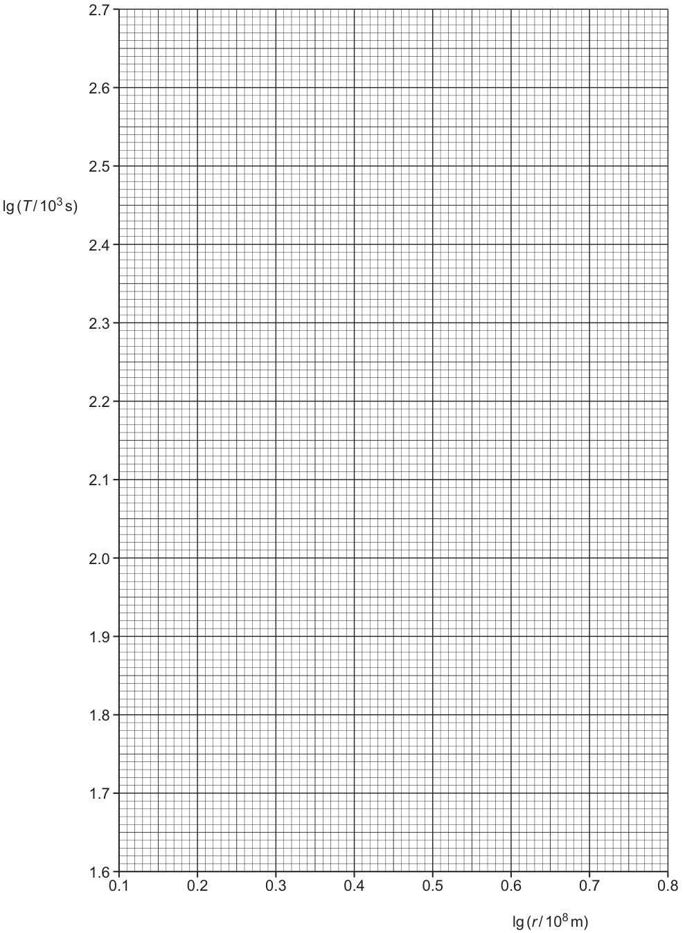
Plot the points where and :
, , , , , .
Add vertical error bars of magnitude at each point:
respectively.
Points plotted with correct vertical error bars (student graph).
Background Concept
A straight-line graph should result if the relationship is a power law. Once the data are converted to
a plot of against can be analysed using a best-fit line.
Error bars represent the uncertainty in each plotted coordinate. Here only has an uncertainty, so only vertical error bars are needed.
Understanding the Question
You must transfer your calculated values from Table 2.1 onto Graph 2.1:
- horizontal axis:
- vertical axis:
and include an error bar on each point equal to the absolute uncertainty in .
Approach
- Mark each point carefully using the grid.
- For each point, draw a vertical line segment from to at the same .
- Keep the error bars thin and accurate so the worst acceptable line can be judged later.
Step-by-Step Reasoning
Use your calculated table values. For example, Pandora is plotted at , .
Its error bar goes from
to
Repeat for all six moons.
A sketch of what you are aiming for (points with vertical error bars and later lines):
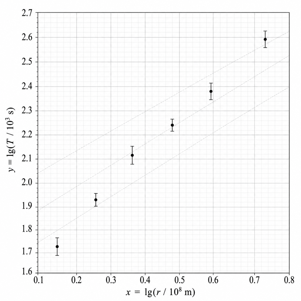
Key Takeaways
- You plot the logarithms (processed values), not the original and .
- Error bars must match the uncertainty in the processed quantity .
Common Mistakes
- Plotting against instead of against .
- Drawing horizontal error bars even though no uncertainty in is given.
- Error bars drawn with the wrong size (e.g. using instead of for Pandora).
Things to Be Careful About
- Plot points to the nearest small square (typical expectation is within about half a small square).
- Ensure axes are labelled exactly with the quantities shown on the printed graph.
- Error bars should be centred on the plotted point (equal length above and below).
Draw the straight line of best fit and a worst acceptable straight line on your graph. Label both lines.
Draw a straight line of best fit through the data (balanced about the points).
Draw a worst acceptable straight line (steepest or shallowest) that still passes through all the vertical error bars.
Label the lines "best fit" and "worst".
Best-fit line and labelled worst acceptable line drawn (student graph).
Background Concept
A best-fit line represents the overall trend in the data. When uncertainties are shown by error bars, you can estimate the uncertainty in the gradient and intercept by drawing a second line (the “worst acceptable line”) that is still consistent with all error bars.
Understanding the Question
You already have a plotted set of points with vertical error bars. Now you must:
- draw the best straight line representing the trend,
- draw one additional straight line that is as different as possible from the best line but still consistent with the error bars,
- label both lines so it is clear which is which.
Approach
- Best fit: aim for roughly equal scatter of points above and below the line.
- Worst acceptable: choose either the steepest or shallowest line that can still pass through every error bar (not necessarily through every central point).
Step-by-Step Reasoning
- Place a ruler so that the line passes through the “middle” of the error bars overall.
- Adjust so that points are reasonably balanced above and below.
- For the worst acceptable line, pivot the ruler to make the gradient as large (or as small) as possible while still intersecting every vertical error bar.
- Clearly write labels on the graph: “best fit” on the main line and “worst” on the other.
Key Takeaways
- Worst acceptable lines must be constrained by error bars, not by the plotted central points.
- Clear labels prevent confusion when reading gradients and intercepts.
Common Mistakes
- Drawing the worst line so that it misses one or more error bars.
- Drawing a curved line (must be straight).
- Forgetting to label the lines.
Things to Be Careful About
- Use the full range of data when judging the fit; don’t force the line through just two points.
- The worst acceptable line should be noticeably different from the best fit, otherwise the uncertainty estimate will be artificially small.
Determine the gradient of the line of best fit. Include the absolute uncertainty in your answer.
gradient = ______
Using two widely separated points on the best-fit line, e.g.
Worst acceptable line gives gradient .
gradient
1.53 ± 0.13
Background Concept
For a straight line , the gradient is
On a plotted graph, you should calculate using two points on the line (not necessarily on data points), chosen far apart to reduce percentage reading error.
To estimate uncertainty in , Paper 5 commonly uses:
where comes from your worst acceptable line.
Understanding the Question
You must read the gradient of your best-fit line on the log-log plot from (c)(i)-(ii) and include an absolute uncertainty by comparing with the worst acceptable line.
Approach
- Pick two points far apart on the best-fit line (use grid intersections if possible).
- Compute .
- Repeat for the worst acceptable line to get .
- Quote .
Step-by-Step Reasoning
- Choose points separated across much of the x-range (e.g. near and ).
- Read values carefully from the grid.
- Compute and and divide.
Using example readings from a suitable best-fit line:
From a worst acceptable line, you might obtain something like . Then
So .
Key Takeaways
- Always use two points on the drawn line, widely separated.
- Uncertainty in gradient comes from comparing best and worst acceptable lines.
Common Mistakes
- Using two adjacent points (large percentage uncertainty).
- Calculating instead of .
- Using points on the data rather than on the best-fit line.
Things to Be Careful About
- Read coordinates to the correct number of small squares.
- Ensure your worst acceptable line genuinely intersects every error bar; otherwise your uncertainty is not valid.
Determine the -intercept of the line of best fit. Include the absolute uncertainty in your answer.
-intercept = ______
From the best-fit line, read the intercept at :
From the worst acceptable line:
-intercept
1.50 ± 0.05
Background Concept
For a straight-line graph , the -intercept is the value of when . Graphically, it is where the line crosses the vertical axis.
With uncertainties and a worst acceptable line, the uncertainty in is commonly estimated by
Understanding the Question
You must obtain the intercept of your best-fit line on the log-log plot, and include an absolute uncertainty using the intercept of the worst acceptable line.
Approach
- Extend the best-fit line to and read off .
- Do the same for the worst acceptable line to get .
- Take the absolute difference as the uncertainty.
Step-by-Step Reasoning
- Make sure you read the intercept from the line, not from a point.
- If the axis does not include clearly, extend the line carefully using a ruler.
Example:
So
Key Takeaways
- Intercept comes from the line crossing .
- Use the same best/worst line method as for gradient uncertainty.
Common Mistakes
- Reading the intercept at the wrong axis value (e.g. confusing with ).
- Not extending the line cleanly with a ruler.
- Using half the difference without being instructed (Paper 5 usually uses the full difference).
Things to Be Careful About
- Quote the intercept to match the scale precision (typically 2 d.p. is enough when grid is 0.1 per major square).
- Use the intercept from the same worst acceptable line you used for the gradient uncertainty (consistent method).
Using your answers to (a), (c)(iii) and (c)(iv), determine the values of and . Include the absolute uncertainties in and . You need not be concerned with units.
= ______
= ______
From (a), gradient so
From (a),
so
Using and ,
Using worst-line values and ,
n = 1.53 ± 0.13; k = (3.5 ± 3.3) × 10^8
Background Concept
After linearising a relationship and plotting a straight-line graph, the gradient and intercept can be linked back to physical constants.
Here, from
you obtain a log form:
where (because of the axis scalings) the intercept is not simply ; it includes extra constants.
If is known, then
(antilog).
Understanding the Question
You are told to use (a), (c)(iii) and (c)(iv):
- from (a) you know how gradient/intercept relate to and ,
- from (c)(iii) you have the measured gradient (and uncertainty),
- from (c)(iv) you have the measured intercept (and uncertainty).
You must calculate numerical values of and , each with an absolute uncertainty.
Approach
- Set equal to the best-fit gradient, and equal to the gradient uncertainty.
- Rearrange the intercept expression to get .
- Convert to with antilog.
- For the uncertainty in , repeat the calculation using the “worst” values (from your worst acceptable line) and take the absolute difference.
Step-by-Step Reasoning
From part (a):
- gradient .
So if your best-fit gradient is with uncertainty ,
For the intercept (part a result):
Rearrange to isolate .
First move terms:
Now take of (a convenient form):
So
hence
Substitute best-fit values (example): , , and :
Then
For uncertainty, repeat with the “worst” line values (the same worst line used for gradient/intercept uncertainties). Example: , :
Absolute uncertainty:
Key Takeaways
- comes directly from the gradient of the log-log plot.
- comes from the intercept, but you must account for the and scalings.
- In Paper 5, uncertainties are commonly found by recalculating using worst-line values.
Common Mistakes
- Using and forgetting the term.
- Using natural log instead of .
- Trying to add percentage uncertainties for without following the best/worst method expected for graph uncertainties.
Things to Be Careful About
- Because contains , even a modest uncertainty in can strongly affect .
- Keep track of which “worst” values you used; use a consistent worst acceptable line for both gradient and intercept.
- When writing in standard form, ensure the power of 10 is correct after antilogging.
Titan is another moon of Saturn. The orbit of Titan has a period of .
Determine the value of for Titan.
= ______
Using
With , and ,
1.2 × 10^9 m
Background Concept
Once a power-law model has been determined, it can be used for prediction. If
then solving for gives
This involves raising a quantity to a non-integer power, so it is best handled with logs or a calculator.
Understanding the Question
Titan’s orbital period is given in seconds. Using your experimentally determined constants and from part (d), you must calculate Titan’s mean orbital radius (in metres).
Approach
- Rearrange the model equation to make the subject.
- Substitute the given period for Titan and your best values of and .
- Calculate and present in standard form.
Step-by-Step Reasoning
Start with
Multiply both sides by :
Raise both sides to the power :
Substitute (example best values): , , :
Evaluating gives approximately
(This is consistent with Titan being much farther from Saturn than the moons in the table.)
Key Takeaways
- Rearranging for requires taking the th root (power ).
- Standard form is appropriate for astronomical distances.
Common Mistakes
- Forgetting to divide by .
- Using instead of power .
- Mixing the scaled quantities from the table (, ) with SI values in this final calculation.
Things to Be Careful About
- Use in seconds as given.
- Use the best estimates of and unless the question explicitly asks for uncertainty in (it does not here).
- Check that your answer is physically reasonable (Titan should have a larger than Rhea, so should exceed about ).