Physics 9702/51 — October/November 2025
Cambridge A-Level · Planning, Analysis and Evaluation · worked solutions for every part, with the mark scheme
Topics Planning · Analysis, Conclusions and Evaluation
On a bench, a steel ball of radius is used to compress a spring by a distance . The ball is held at rest in this position, as shown in Fig. 1.1.
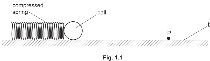
The ball is released and rolls along the bench. At a fixed point P, the ball has speed . The speed of the ball at P is determined using one light gate connected to a timer.
Several steel balls of different radii are available.
It is suggested that is related to by the relationship
where is the spring constant of the spring, is the density of the steel, and and are constants.
Plan a laboratory experiment to test the relationship between and .
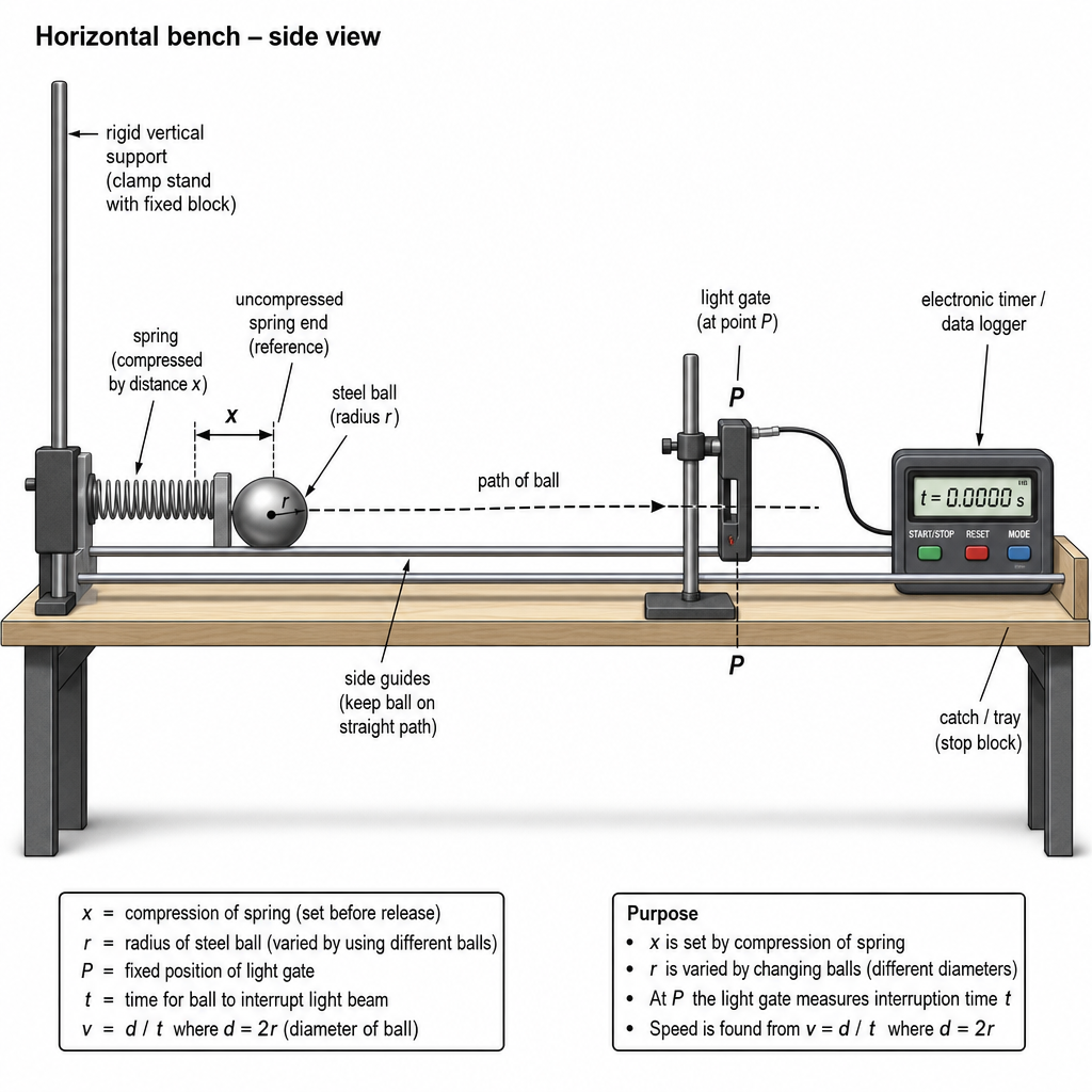
Draw a diagram showing the arrangement of your equipment.
Explain how the results could be used to determine values for and .
In your plan you should include:
- the procedure to be followed
- the measurements to be taken
- the control of variables
- the analysis of the data
- any safety precautions to be taken.
Answer
Variables
- Independent variable: ball radius (use several steel balls of different radii).
- Dependent variable: speed at fixed point .
- Controlled: compression , spring and spring constant , position of light gate at , bench level/surface, release method, same rolling path (no slipping).
Apparatus
Spring and clamp/rigid stop, metre rule, set square/marker for fixed compression, several steel balls, micrometer screw gauge/vernier calipers, light gate + timer/data logger, retort stands/clamps, tray/stop to catch ball.
Procedure and measurements
- Fix the spring against a rigid support on the bench. Mark a fixed point on the bench and clamp a light gate at .
- Set a fixed compression using a metre rule and a stop/marker so the spring is compressed by the same amount each run.
- For each ball:
- Measure its diameter with a micrometer (several orientations), calculate .
- Place the ball against the compressed spring and release without pushing.
- Record the time for which the light beam is interrupted as the ball passes through the light gate at .
- Repeat at least 3 times and average .
- Calculate the speed at using
and hence calculate .
Analysis to determine and
Given
Take logs:
- Plot (y-axis) against (x-axis).
- Gradient so .
- Intercept so
and hence
(using known for steel, measured/known , and fixed measured ).
Control of variables (examples)
- Use the same spring throughout; do not change its extension range.
- Keep fixed using a physical stop; check with ruler each run.
- Keep light gate at the same point and same height so the ball passes centrally.
- Ensure bench is horizontal and surface condition unchanged.
- Use side guides to keep the ball travelling straight and rolling without slipping.
Safety
- Prevent ball falling off the bench: use a tray/stop at the end; keep feet clear.
- Keep fingers clear of the compressed spring when releasing; ensure clamp/support is secure.
- Ensure stands and light gate are stable to avoid toppling.
See working
Background Concept
The suggested relationship is a power law connecting the ball speed at a fixed position to its radius :
Here is the spring constant, is the compression (so the spring energy depends on ), is the density of steel (constant for all the balls), and and are unknown constants.
To "test the relationship" you need to vary systematically, measure , and then check whether the data fit the functional form. For power laws, the standard method is to take logarithms so that the relationship becomes linear, allowing the constants to be found from a straight-line graph.
A light gate measures the time interval for which its beam is blocked. If the moving object blocks a known length , then
For a sphere passing through a narrow light beam, the blocked length along the direction of motion is approximately the diameter , so .
Understanding the Question
You have a spring that launches a steel ball by releasing it from a fixed compression . The ball then rolls along the bench and passes a single light gate at point , where its speed is .
You are given multiple balls with different radii . You must plan an experiment that:
- varies (independent variable),
- measures at (dependent variable) using one light gate,
- keeps other quantities constant (especially and the setup),
- uses the results to determine and .
Because the equation contains and , the natural analysis is a log-log plot.
Approach
- Set up the apparatus so that the spring compression is the same each trial and the light gate stays fixed at .
- For each ball, measure accurately using a micrometer or vernier calipers.
- Use the light gate to measure the interruption time as the ball passes; use the diameter as the distance that blocks the beam, and calculate .
- Calculate for each ball.
- Linearise the relationship by taking logs and plot against . The gradient gives , and the intercept gives , from which can be calculated.
- Include practical steps to reduce uncertainty (repeat timings, ensure straight rolling, stable clamping) and include safety measures.
Step-by-Step Reasoning
1) Setting the spring compression as a constant
Since appears squared, even a small change in would significantly change . So you should fix using a physical stop (e.g. a block or pin position) and confirm with a ruler.
2) Measuring the independent variable
Measure the ball diameter with a micrometer screw gauge (best precision). Take readings in several orientations (to check it is spherical) and average. Then
3) Measuring speed with one light gate
When the sphere passes through the light gate, it blocks the beam for time . The distance corresponding to the blocked beam is the sphere diameter (along the direction of travel), so
To reduce random timing scatter, repeat the run several times for each ball and average .
4) Linearising to find
Start from:
Take natural logs:
This matches the straight-line form if you identify:
- gradient
- intercept
So:
- Find the best-fit straight line and its gradient ; then .
5) Using the intercept to find
From the intercept:
Rearrange:
You can use a known value of for steel (or measure it separately if required), and obtain from prior calibration of the spring (or given). Since is set and measured, you can calculate .
6) Control of variables (what matters and why)
- Same spring / same : changing spring changes the energy delivered.
- Same compression : directly affects via .
- Same point and gate alignment: ensures speed is measured at the same location each time.
- Bench level and same surface: changes in slope or friction would change .
- Ensure rolling without slipping: slipping changes the energy distribution and can alter the relationship.
7) Safety
Main hazards are the ball leaving the bench and the spring snapping forward. A catching tray/stop and careful hand placement (or a mechanical release) address these.
Key Takeaways
- A single light gate can measure speed if the interrupted length is known (here, the ball diameter).
- To test a power law , use a log-log plot to obtain a straight line.
- Gradient gives the exponent () and intercept gives the constant (here used to find ).
- Good planning depends on identifying and controlling the variables that appear in the model equation.
Common Mistakes
- Not keeping constant (or not explaining how it is kept constant).
- Measuring only one timing per ball (insufficient repeats for reliability).
- Plotting against directly and trying to guess (won’t reliably extract the exponent).
- Using the wrong distance in (must use the diameter , not the radius).
- Forgetting that the gradient is negative: , not .
Things to Be Careful About
- The beam must be narrow and the ball must pass centrally; otherwise the blocked length may differ slightly from .
- Use consistent units for throughout (e.g. convert mm to m before logging if you want SI consistency).
- When taking logs, any base is acceptable provided it is used consistently; if using , then and you must use rather than .
- Ensure the ball is released without an extra push; a mechanical release improves consistency.
- If the bench is not horizontal, gravitational potential energy changes between runs and can distort the results.
A student investigates light from different galaxies.
Fig. 2.1 shows the lines in the absorption spectrum from a distant galaxy.
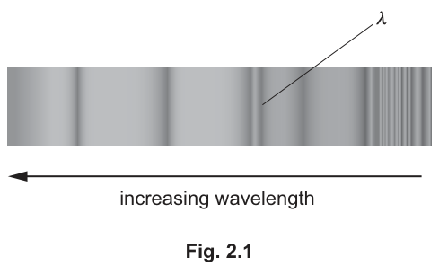
The wavelength of one of the lines in the absorption spectrum is . The wavelength of this spectral line in the laboratory is .
The observations of the same spectral line are repeated for different galaxies.
The student determines the distance of each galaxy from the Earth.
It is suggested that and are related by the equation
where is the speed of light in free space and is the Hubble constant.
A graph is plotted of on the -axis against on the -axis.
Determine expressions for the gradient and -intercept.
gradient = ______
-intercept = ______
Working
Given
so
Answer
Gradient
-intercept
Gradient = λ0H; y-intercept = λ0
Background Concept
Hubble’s law in this question is written in terms of fractional wavelength shift (redshift):
This is the observed change in wavelength relative to the laboratory (rest) wavelength. If this redshift is proportional to distance, then we expect a straight-line relationship when we plot suitable variables.
A straight-line graph has the form
where is the gradient and is the -intercept.
Understanding the Question
You are told that
and you are plotting on the -axis against on the -axis.
So you must rewrite the equation into the form:
Then the coefficient of is the gradient, and the constant term is the intercept.
Approach
- Multiply both sides by to remove the fraction.
- Rearrange to make the subject.
- Compare with where and .
Step-by-Step Reasoning
Start with
Multiply by :
Recognise that is the -axis variable:
Add to both sides:
Comparing with :
- gradient
- -intercept
Key Takeaways
- To find gradient and intercept, rewrite into using the variables actually plotted.
- The intercept often represents the value of when (here, when ).
Common Mistakes
- Giving gradient as instead of .
- Not fully rearranging to make the subject.
- Treating (instead of ) as the -variable.
Things to Be Careful About
- Make sure the plotted -variable matches the algebra exactly (here it is ).
- Do not confuse the constant (speed of light) with the intercept in ; they are different symbols with different meanings.
Values of and are given in Table 2.1.
Table 2.1
The value of is .
Calculate and record values of in Table 2.1. Include the absolute uncertainties in .
Working
For each galaxy,
Uncertainty:
Values (in ):
- :
- :
- :
- :
- :
- :
Answer
d/c / 10^15 s = 1.60±0.40, 3.47±0.40, 4.83±0.40, 6.00±0.40, 9.50±0.40, 12.5±0.40
Background Concept
The quantity has units of time because
If is treated as an exact constant, then dividing by scales both the value and the absolute uncertainty in by the same factor:
Understanding the Question
You are given distances (each with absolute uncertainty ) and must compute the corresponding -axis quantity for the graph:
and record it in the table as , including the absolute uncertainty.
Approach
For each row:
- Convert into km using the scale factor .
- Divide by .
- Express the result in units of .
- Propagate uncertainty using .
Step-by-Step Reasoning
Example for the first distance:
Compute time:
Uncertainty in is . Divide by the same :
This uncertainty is the same for every row because is the same for every row.
Key Takeaways
- Dividing a measured quantity by an exact constant divides both the value and absolute uncertainty by that constant.
- Keep table entries to consistent decimal places/precision.
Common Mistakes
- Using percentage uncertainty incorrectly; here absolute uncertainty is simplest: .
- Forgetting to apply the powers of ten ( and ).
- Mixing units (e.g. using in while is in km).
Things to Be Careful About
- Ensure is used as since is in km.
- When writing in the table column headed , you must scale both the central value and its uncertainty by .
Answer
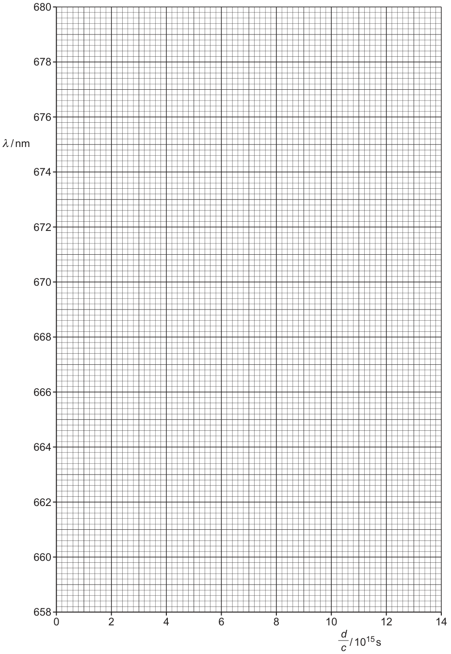
Plot the six points where and .
Draw horizontal error bars of in for each point.
See graph
Background Concept
A good graph in Paper 5 must:
- have correctly labelled axes with quantities and units,
- use a sensible linear scale (typically using at least half the grid in each direction),
- plot points accurately,
- include error bars when uncertainties are given.
Error bars show the range in which the true value could lie. Here only has an uncertainty, so the error bars are horizontal.
Understanding the Question
You are asked to plot:
- -axis:
- -axis:
using the calculated -values from part (b) and the given wavelengths.
You must include error bars for , i.e. on the -coordinate of each point. From (b) these are (in the plotted units).
Approach
- Transfer each pair from the table to the grid.
- Plot each point with a small, clear cross or dot.
- For each point, add an error bar extending left and right by along the -direction.
Step-by-Step Reasoning
The six -values (in units of ) are approximately:
.
For each plotted point:
- locate the position,
- locate the position using the corresponding value,
- draw a horizontal line segment from to at that same level (often with small vertical end-caps).
Key Takeaways
- Only draw error bars in the direction(s) where uncertainties are provided.
- Use the graph paper efficiently: clear points, clear error bars, clear axis labels.
Common Mistakes
- Drawing vertical error bars in when no uncertainty is given.
- Using the uncertainty in instead of the uncertainty in (the plotted quantity).
- Plotting on the -axis instead of .
Things to Be Careful About
- The table heading is , so the uncertainty is also in those units ().
- Points should be fine enough that a best-fit line can be drawn through the trend (avoid large blobs).
Draw the straight line of best fit and a worst acceptable straight line on your graph. Label both lines.
Answer
Draw a single straight line of best fit through the points.
Draw a worst acceptable straight line (steepest or shallowest line that still passes through all the error bars).
Label both lines on the graph.
See graph
Background Concept
- A line of best fit is drawn to represent the overall linear trend, with roughly equal scatter of points above and below the line.
- A worst acceptable line (sometimes called a worst-fit line) is used to estimate uncertainty in the gradient and intercept. It should be the steepest or shallowest straight line that is still consistent with the data within their error bars.
Understanding the Question
You already plotted points and horizontal error bars in (c)(i). Now you must draw:
- the best-fit straight line;
- one worst acceptable straight line;
and label them.
Approach
- Use a ruler to draw the best-fit line through the main trend (not joining dot-to-dot).
- Decide whether the steepest or shallowest line gives the bigger difference in gradient from the best-fit value.
- Draw that extreme line ensuring every point’s error bar is intersected by the line (or at least all points are consistent within uncertainties).
Step-by-Step Reasoning
- For the best-fit line, aim for a balanced distribution: do not force the line through every point.
- For the worst acceptable line, imagine “tilting” the line about some central region until it is just about to miss an error bar at one end while still intersecting the error bars at the other end. The idea is to make the gradient as different as possible but still plausible.
Label them clearly, e.g. “best fit” and “worst acceptable”.
Key Takeaways
- Worst acceptable lines are a graphical way to estimate uncertainty without formal statistics.
- Error bars define what is “acceptable”.
Common Mistakes
- Drawing a worst line that misses one or more error bars.
- Drawing two worst lines when only one is requested.
- Joining points with segments instead of drawing a single straight best-fit line.
Things to Be Careful About
- Because the uncertainties here are horizontal, the line must intersect each point’s horizontal error bar region.
- Always use a long triangle when finding gradients later, so draw the lines long enough across the graph.
Determine the gradient of the line of best fit. Include the absolute uncertainty in your answer.
gradient = ______
Working
From the best-fit line,
From the worst acceptable line,
Answer
(1.83 ± 0.21) nm (10^15 s)^{-1}
Background Concept
The gradient of a straight line is
To reduce percentage reading error, choose two points on the line that are far apart (a “large triangle”), rather than using adjacent grid squares.
Graphical uncertainty method (Paper 5):
- find from the best-fit line,
- find from the worst acceptable line,
- take
Understanding the Question
You must read the gradient of the best-fit line you drew on Graph 2.1, and include an absolute uncertainty using your worst acceptable line.
Units: since is in nm and is in , the gradient unit is
Approach
- Pick two well-separated points on the best-fit line and compute .
- Pick two well-separated points on the worst acceptable line and compute .
- Uncertainty is the absolute difference.
Step-by-Step Reasoning
Using the linear trend in the plotted data, a typical best-fit gradient is about
A plausible worst acceptable gradient (steepest acceptable) is about
So
(If your worst line is the shallowest acceptable, you would compare to that instead; you choose the one that gives the larger difference.)
Key Takeaways
- Always use from two far-apart points on the line.
- Uncertainty in gradient comes from comparing best vs worst acceptable lines.
Common Mistakes
- Using two plotted points instead of two points on the best-fit line.
- Calculating by accident.
- Quoting uncertainty as half the range instead of (Cambridge typically uses the absolute difference).
Things to Be Careful About
- Read coordinates carefully from the axes; include the correct scale factor ( is already built into the axis label).
- Quote uncertainty as an absolute uncertainty with the same unit as the gradient.
Determine the -intercept of the line of best fit. Include the absolute uncertainty in your answer.
-intercept = ______
Working
From the best-fit line,
From the worst acceptable line,
Answer
(655.1 ± 1.2) nm
Background Concept
For a straight line
the -intercept is the value of when .
Graphical uncertainty method is the same idea as for the gradient:
Understanding the Question
You must find the intercept of your best-fit line on the graph of (nm) against . This intercept will later be used to find .
Approach
- Extend the best-fit line back to if necessary.
- Read off the value where it crosses the -axis.
- Do the same for the worst acceptable line.
- Take the absolute difference as the uncertainty.
Step-by-Step Reasoning
From the linear trend, the best-fit line typically crosses the -axis at about
A plausible worst-line intercept is around
so
Hence
Key Takeaways
- The intercept is a read-off at from the line, not from a data point.
- Worst acceptable line provides the uncertainty estimate.
Common Mistakes
- Reading the intercept from the grid using a plotted point near the axis rather than the drawn line.
- Forgetting to extend the line to reach .
- Quoting uncertainty with the wrong unit or as a percentage.
Things to Be Careful About
- Keep the same decimal precision as justified by graph-reading (often 0.1 nm is acceptable if the scale allows).
- The intercept uncertainty should come from your own worst acceptable line, not an arbitrary guess.
Using your answers to (a), (c)(iii) and (c)(iv), determine the values of and . Include appropriate units.
= ______
= ______
Working
From (a), intercept .
So
From (a), true gradient (for plot of vs ) is .
But the graph uses
So
Hence plotted gradient
so
Using and :
Fractional uncertainty:
Answer
λ0 = (655.1 ± 1.2) nm; H = (2.8 ± 0.3) × 10^-18 s^-1
Background Concept
From part (a), when you plot against , the straight-line form is
So:
- intercept
- gradient (with in seconds)
However, if the graph’s -axis uses a scaled variable (here ), then the plotted gradient is different by a scale factor.
For uncertainties in products/quotients, add fractional uncertainties:
Understanding the Question
You must use:
- your intercept from (c)(iv) to obtain ,
- your gradient from (c)(iii) (including its uncertainty) to obtain .
You must include appropriate units.
Approach
- Set equal to the intercept (and keep its uncertainty).
- Correctly relate the plotted gradient to the theoretical gradient, accounting for the scaling on the -axis.
- Solve for .
- Propagate uncertainties using fractional uncertainty addition.
Step-by-Step Reasoning
From (a): intercept .
So directly:
Now handle the gradient carefully.
The theory says
But the plotted variable is
so . Substitute:
Comparing with gives
Therefore
Using and :
Uncertainty:
So
Key Takeaways
- Intercept often gives the “zero-distance” (rest) value .
- Always account for axis scaling factors when converting gradients into physical constants.
- Fractional uncertainties add for multiplication/division.
Common Mistakes
- Forgetting the scale factor and using (this gives a value too large by ).
- Mixing units for wavelength (nm vs m). Here it is safe to keep nm because the ratio cancels the length unit.
- Combining uncertainties incorrectly (e.g. subtracting fractional uncertainties).
Things to Be Careful About
- Quote with unit .
- Keep consistency: if you keep wavelengths in nm, keep both gradient and intercept in nm so the ratio is dimensionless before applying .
Hubble’s law suggests that the age of the universe is related to by
Determine a value for . Include the absolute uncertainty in your answer.
= ______
Working
Using :
For ,
so
Answer
(3.6 ± 0.4) × 10^17 s
Background Concept
If
then is the reciprocal of . For uncertainty propagation:
- for , the fractional uncertainty is unchanged:
This comes from differentiating (or from standard uncertainty rules).
Understanding the Question
You have obtained (with an absolute uncertainty) in part (d). You must compute
and include an absolute uncertainty in , with unit seconds.
Approach
- Calculate using the central value of .
- Find the fractional uncertainty .
- Apply the same fractional uncertainty to to get .
Step-by-Step Reasoning
Using :
Central value:
Fractional uncertainty:
So
Therefore
Key Takeaways
- Taking a reciprocal does not change the fractional uncertainty.
- Convert the fractional uncertainty back to an absolute uncertainty at the end.
Common Mistakes
- Using (incorrect).
- Forgetting that is in so must be in .
- Rounding too aggressively compared with its uncertainty.
Things to Be Careful About
- Quote and to consistent significant figures (typically match the uncertainty to 1 s.f. or 2 s.f., then match the value accordingly).
- Keep standard form clear: is preferable to writing two separate powers of ten.