Physics 9702/54 — May/June 2025

Cambridge A-Level · Planning, Analysis and Evaluation · worked solutions for every part, with the mark scheme

questions

marks

minutes

Topics Analysis, Conclusions and Evaluation · Planning

Q115MMedium-HardPlanningAnalysis, Conclusions and Evaluation

A ball is dropped on to an inclined thin metal sheet, as shown in Fig. 1.1.

Fig. 1.1

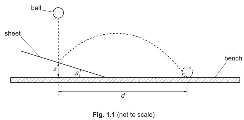
The angle between the sheet and the horizontal bench is $\theta$ . The height of the point of contact of the ball and the sheet is $z$ . The horizontal distance travelled by the ball between its points of contact with the sheet and the bench is $d$ , as shown in Fig. 1.1.

It is suggested that $d$ is related to $\theta$ by the relationship

d = \frac{Pv^2 \sin 4\theta}{g} + Q\sqrt{z}

where $v$ is the speed of the ball as it makes contact with the sheet, $g$ is the acceleration of free fall, and $P$ and $Q$ are constants.

Plan a laboratory experiment to test the relationship between $d$ and $\theta$ .

Draw a diagram showing the arrangement of your equipment.

Explain how the results could be used to determine values for $P$ and $Q$ .

In your plan you should include:

the procedure to be followed
the measurements to be taken
the control of variables
the analysis of the data
any safety precautions to be taken.

Diagram

Diagram Space

DifficultyMedium-Hard

Worked solution

Variables

Independent variable: $\theta$ .
Dependent variable: $d$ .
Control variables: $v$ (by keeping drop height $h$ constant), $z$ (keep point of impact fixed in space), same ball, same sheet/surface condition, same release method (no push/spin).

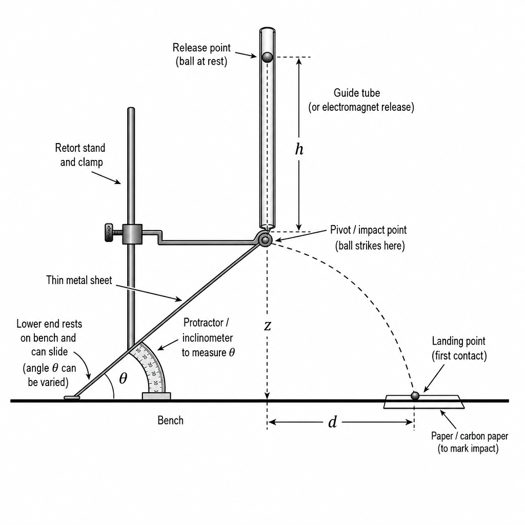
Diagram / arrangement

diagram-1

Procedure and measurements

Fix a thin metal sheet so it can rotate about a pivot at the chosen impact point (so the impact point stays at constant height $z$ above the bench). Adjust the lower end on the bench to set different angles.
Measure $z$ (vertical height of the impact point above the bench) with a metre rule/set square; keep it constant throughout.
Set up a vertical guide tube (or electromagnet release) directly above the impact point and release the same ball from rest from a fixed height. Measure the vertical drop distance $h$ from release point to the impact point; keep $h$ constant.
For a chosen $\theta$ (measure with protractor/inclinometer), release the ball so it strikes the marked point on the sheet.
Mark the landing point on the bench using paper/carbon paper. Measure the horizontal distance $d$ from the vertical line through the impact point to the landing mark using a metre rule.
Repeat at least 3 times for each $\theta$ and take the mean $d$ .
Repeat for at least 6 different values of $\theta$ over a suitable range (e.g. $10^\circ$ to $40^\circ$ ) so that $\sin 4\theta$ varies substantially.

Analysis (to find $P$ and $Q$ )

Calculate $v$ using free-fall:

v^2 = 2gh

From

d = \frac{Pv^2}{g}\sin 4\theta + Q\sqrt{z}

with $v$ and $z$ constant, plot a graph of $d$ (y-axis) against $\sin 4\theta$ (x-axis).

Gradient $m = \frac{Pv^2}{g}$ so

P = \frac{mg}{v^2}

Intercept $c = Q\sqrt{z}$ so

Q = \frac{c}{\sqrt{z}}

A straight line confirms the suggested relationship (within experimental uncertainty).

Safety

Prevent the ball from bouncing into walkways: use a catch tray/side barriers and keep the area clear.
Ensure the sheet and clamp stand are stable/weighted so they cannot tip when struck.
Keep fingers/feet clear of the landing region; eye protection is advisable.

Final answer

See working

Detailed explanation

Background Concept

The suggested relationship is

d = \frac{Pv^2 \sin 4\theta}{g} + Q\sqrt{z}

This has the structure

d = A\sin 4\theta + B

where

A = \frac{Pv^2}{g}, \qquad B = Q\sqrt{z}.

If we can keep $v$ and $z$ constant while varying $\theta$ , then $A$ and $B$ are constants and a plot of $d$ against $\sin 4\theta$ should be a straight line.

The speed $v$ as the ball reaches the sheet can be made known and constant by dropping it from rest through a fixed vertical height $h$ above the impact point. Neglecting air resistance,

v^2 = u^2 + 2gh \;\Rightarrow\; v^2 = 2gh \quad (u=0).

Understanding the Question

You are asked to plan an experiment that tests whether $d$ depends on $\theta$ according to the given equation, and then to explain how to use the data to find numerical values for the constants $P$ and $Q$ .

So you must:

vary $\theta$ systematically,
measure $d$ for each $\theta$ ,
keep other quantities in the equation under control (especially $v$ and $z$ ),
choose a graph/analysis that turns the equation into a straight-line form so that gradient and intercept give $P$ and $Q$ .

Approach

Choose $\theta$ as the independent variable and $d$ as the dependent variable.
Make $v$ constant by using the same ball and the same release height $h$ above the impact point (a guide tube helps ensure no sideways launch speed).
Make $z$ constant by ensuring the point where the ball hits the sheet stays at the same height above the bench even when the sheet angle changes. The simplest way is to pivot/hinge the sheet about the impact point.
For each $\theta$ , measure $d$ and compute $\sin 4\theta$ .
Plot $d$ against $\sin 4\theta$ ; use gradient and intercept to determine $P$ and $Q$ .

Step-by-Step Reasoning

diagram-1

(1) Setting the geometry and keeping $z$ constant

A common pitfall is that if you simply raise one end of the sheet, the impact point moves up/down and $z$ changes with $\theta$ . That would change the $Q\sqrt{z}$ term and destroy the simple linear test.

To avoid this, fix the sheet so it rotates about a pivot located exactly at the chosen impact point. Then, when you change $\theta$ , the impact point stays at the same position in space, so $z$ remains constant.

Measure $z$ once (vertical height from bench to the impact point). You can use a set square with a metre rule to measure vertical height reliably.

(2) Making $v$ known and constant

Release the ball from rest from a fixed vertical height $h$ above the impact point. Using a tube ensures the ball falls vertically and hits the same point each time.

Measure $h$ and use

v^2 = 2gh.

Since $h$ is fixed, $v$ is fixed for all trials.

(3) Measuring $d$ reliably

For each $\theta$ :

measure $\theta$ with a protractor/inclinometer (repeat or check for parallax),
drop the ball and mark the first contact point on the bench (paper/carbon paper helps),
measure horizontal distance $d$ from the vertical line under the impact point to the landing mark.

Repeat the drop several times at each $\theta$ and take the mean $d$ to reduce random effects (slightly different bounces, small changes in impact point, etc.).

(4) Linear graph and extracting $P$ and $Q$

With $v$ and $z$ constant, rewrite the equation as

d = \left(\frac{Pv^2}{g}\right)\sin 4\theta + Q\sqrt{z}.

So if you define

x = \sin 4\theta, \qquad y = d,

you have

y = mx + c

with

m = \frac{Pv^2}{g}, \qquad c = Q\sqrt{z}.

From the graph:

Determine the gradient $m$ using a large triangle, then calculate

P = \frac{mg}{v^2}.

Read the y-intercept $c$ , then calculate

Q = \frac{c}{\sqrt{z}}.

A straight line (within scatter) supports the proposed relationship.

Key Takeaways

In planning questions, success depends on choosing the correct independent variable and controlling everything else in the given equation.
To test a relationship efficiently, convert it to a straight-line form and choose a graph where gradient/intercept directly yield the constants.
A practical plan must include repeat readings, a clear method for measuring each quantity, and explicit control of variables.

Common Mistakes

Letting $z$ change when changing $\theta$ (then the intercept term is not constant and the graph may curve).
Not stating how $v$ is kept constant/known (it is in the equation, so it must be controlled or measured).
Plotting $d$ against $\theta$ instead of $\sin 4\theta$ (does not linearise the relationship).
Using too small a range of $\theta$ so $\sin 4\theta$ hardly changes, giving a very uncertain gradient.
Not repeating measurements or not stating averaging.

Things to Be Careful About

Ensure the ball hits the same point on the sheet each time (mark the point and use a guide tube); otherwise $z$ and the effective bounce conditions can vary.
Choose $\theta$ values where $\sin 4\theta$ varies smoothly and avoids extreme sensitivity near where the slope of $\sin 4\theta$ changes rapidly.
Measure $d$ horizontally (not along the sheet or along the projectile path) and define the reference line (vertical below impact point) clearly.
Keep the apparatus stable: an unsecured sheet changes angle on impact, changing $\theta$ during the bounce.
Record units consistently (e.g. $d$ in $\text{m}$ , $z$ and $h$ in $\text{m}$ ) before using the formulas.

Techniques used

identify independent, dependent and control variables from a proposed relationshipdesign a method to vary the angle while holding other quantities constantlinearise the relationship by choosing a suitable graphuse gradient and intercept to determine constantsreduce random error by repeating measurements and averaging

Answer

Gradient (= n)

(y)-intercept (= \lg k)

Final answer

gradient = n, y-intercept = lg k

Detailed explanation

Background Concept

A power law

\lambda = k\mu^n

can be tested using a straight-line graph by taking logarithms (base 10 here). Using log laws:

\lg(AB)=\lg A + \lg B, \qquad \lg(A^n)=n\lg A.

This converts the power law into the straight-line form

y = mx + c,

where the gradient (m) and intercept (c) can be read from the graph.

Understanding the Question

You are told the suggested relationship between relative luminosity (\lambda) and relative mass (\mu) is (\lambda = k\mu^n). A graph is plotted of (\lg \lambda) (vertical axis) against (\lg \mu) (horizontal axis). You must state what the gradient and the (y)-intercept represent in terms of (k) and (n).

Approach

Take (\lg) of both sides of (\lambda = k\mu^n).
Use log laws to separate into a sum.
Compare with (y = mx + c) where (y = \lg\lambda) and (x = \lg\mu).

Step-by-Step Reasoning

Start with

\lambda = k\mu^n.

Take (\lg) of both sides:

\lg\lambda = \lg(k\mu^n).

Use (\lg(AB)=\lg A + \lg B) and (\lg(A^n)=n\lg A):

\lg\lambda = \lg k + \lg(\mu^n)=\lg k + n\lg\mu.

Now identify the straight-line form:

(y = \lg\lambda)
(x = \lg\mu)
gradient (m = n)
intercept (c = \lg k)

Key Takeaways

Taking logarithms linearises power laws.
On a (\lg y) vs (\lg x) plot, the gradient gives the power (n) and the intercept gives (\lg k).

Common Mistakes

Writing the intercept as (k) instead of (\lg k).
Forgetting that the plotted variables are (\lg \lambda) and (\lg \mu), not (\lambda) and (\mu).

Things to Be Careful About

The base of the logarithm matters: (\lg) means base 10, so the intercept corresponds to (\lg k), and later (k) is found using (k = 10^{\text{intercept}}).

Techniques used

take logarithms to linearise a power lawmatch a linearised equation to y = mx + cidentify gradient and intercept from the linear form

(b)

Values of $\mu$ and $\lambda$ are given in Table 2.1.

Table 2.1

$\mu$	$\lambda$	$\lg \mu$	$\lg \lambda$
$4.6 \pm 0.4$	$500$
$5.4 \pm 0.4$	$800$
$8.4 \pm 0.4$	$3200$
$11 \pm 1$	$7000$
$16 \pm 1$	$25000$
$18 \pm 1$	$38000$

Calculate and record values of $\lg \mu$ and $\lg \lambda$ in Table 2.1.
Include the absolute uncertainties in $\lg \mu$ .

2M Similar

DifficultyMedium

Worked solution

For (x=\lg \mu), absolute uncertainty:

\Delta(\lg\mu)=\frac{1}{\ln 10}\frac{\Delta\mu}{\mu}=0.434\,\frac{\Delta\mu}{\mu}

Calculated values (3 d.p.):

(\mu)	(\lambda)	(\lg\mu)	(\Delta(\lg\mu))	(\lg\lambda)
4.6 (\pm 0.4)	500	0.663	0.038	2.699
5.4 (\pm 0.4)	800	0.732	0.032	2.903
8.4 (\pm 0.4)	3200	0.924	0.021	3.505
11 (\pm 1)	7000	1.041	0.039	3.845
16 (\pm 1)	25000	1.204	0.027	4.398
18 (\pm 1)	38000	1.255	0.024	4.580

Final answer

lgμ and lgλ values with Δ(lgμ) as in table

Detailed explanation

Background Concept

When you transform data using a function (here (\lg)), uncertainties also transform.

For a small uncertainty (\Delta\mu), the uncertainty in (\lg\mu) can be found using differentials:

\Delta(\lg\mu) \approx \left|\frac{\mathrm{d}(\lg\mu)}{\mathrm{d}\mu}\right|\Delta\mu.

Since

\lg\mu = \frac{\ln\mu}{\ln 10},

we have

\frac{\mathrm{d}(\lg\mu)}{\mathrm{d}\mu} = \frac{1}{\ln 10}\frac{1}{\mu}.

\Delta(\lg\mu) = \frac{1}{\ln 10}\frac{\Delta\mu}{\mu} \approx 0.434\,\frac{\Delta\mu}{\mu}.

This is why horizontal error bars on a (\lg\mu) axis are based on the fractional uncertainty in (\mu).

Understanding the Question

You are given six values of relative mass (\mu) with uncertainties, and six values of relative luminosity (\lambda) (no uncertainties given). You must:

compute (\lg\mu) for each star,
compute (\lg\lambda) for each star,
and include the absolute uncertainty in (\lg\mu) (so you can later draw error bars in (x)).

Approach

For each row:

Calculate (\lg\mu) using a calculator.
Calculate (\lg\lambda).
Convert (\Delta\mu) to (\Delta(\lg\mu)) using

\Delta(\lg\mu)=0.434\,\frac{\Delta\mu}{\mu}.

Record values to consistent decimal places (typically 3 d.p. for logs here, since the uncertainties are a few (\times 10^{-2})).

Step-by-Step Reasoning

Example (first row): (\mu = 4.6 \pm 0.4).

Log value:

\lg\mu = \lg(4.6)=0.6628\approx 0.663.

Uncertainty:

\Delta(\lg\mu)=0.434\,\frac{0.4}{4.6}=0.0377\approx 0.038.

For (\lambda=500):

\lg\lambda = \lg(500)=2.699.

Repeat the same process for each row. Notice that as (\mu) increases, the fractional uncertainty (\Delta\mu/\mu) generally decreases, so (\Delta(\lg\mu)) decreases.

Key Takeaways

(\lg) values should be recorded consistently (same d.p. across a column).
For logs, absolute uncertainty depends on fractional uncertainty: (\Delta(\lg\mu)\propto \Delta\mu/\mu).

Common Mistakes

Using (\Delta(\lg\mu)=\lg(\Delta\mu)) (wrong).
Forgetting the factor (1/\ln 10) (i.e. using (\Delta\mu/\mu) directly).
Writing uncertainties to too many decimal places or inconsistent d.p.

Things to Be Careful About

Use (\ln) (natural log) in the uncertainty formula even though the graph uses (\lg): the conversion factor (1/\ln 10) is essential.
Keep an appropriate number of significant figures: uncertainties like (0.038) justify giving (\lg\mu) to 3 d.p. rather than 2 d.p.

Techniques used

calculate common logarithms of measured quantitiespropagate an absolute uncertainty through a logarithmrecord values to consistent decimal places

(c)

(i)

Plot a graph of $\lg \lambda$ against $\lg \mu$ .
Include error bars for $\lg \mu$ .

Graph Paper

2M Similar

DifficultyMedium-Easy

Worked solution

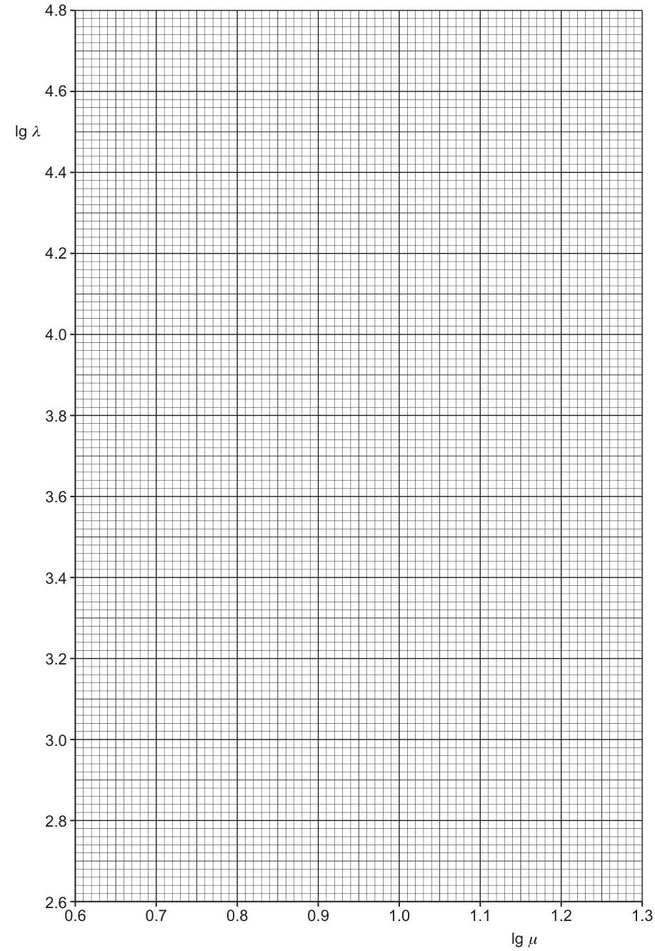
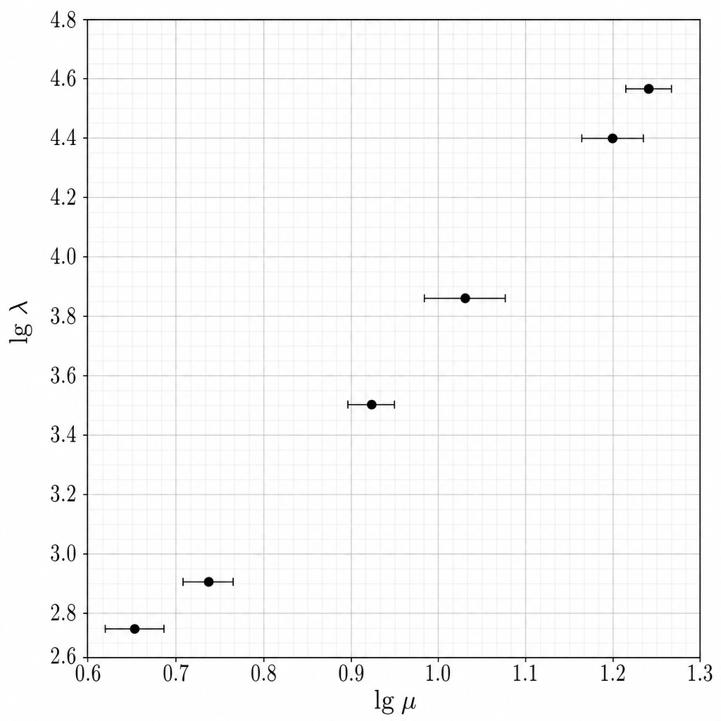
Plot the points ((x=\lg\mu,, y=\lg\lambda)) (from part (b)):

((0.663,,2.699)), ((0.732,,2.903)), ((0.924,,3.505)), ((1.041,,3.845)), ((1.204,,4.398)), ((1.255,,4.580)).

Add horizontal error bars of (\pm\Delta(\lg\mu)): (\pm0.038,\pm0.032,\pm0.021,\pm0.039,\pm0.027,\pm0.024) respectively.

Answer

Graph of (\lg\lambda) against (\lg\mu) with correct points and (x)-error bars plotted.

Final answer

Correct plot with x-error bars

Detailed explanation

Background Concept

To test (\lambda = k\mu^n), we plot

\lg\lambda = n\lg\mu + \lg k

so a straight-line trend supports the power law. Uncertainties in (\mu) become uncertainties in (x=\lg\mu), shown as horizontal error bars of size (\pm\Delta(\lg\mu)).

Understanding the Question

You must place six points on a grid where:

the horizontal axis is (x=\lg\mu),
the vertical axis is (y=\lg\lambda),
and each point has a horizontal error bar only (because only (\mu) has uncertainty).

Approach

Use the calculated coordinates from part (b).
Plot each point accurately.
For each point, draw a horizontal error bar from (x-\Delta x) to (x+\Delta x) where (\Delta x = \Delta(\lg\mu)).
Ensure axes labels include the correct quantities ((\lg\lambda) and (\lg\mu)).

Step-by-Step Reasoning

The coordinates come directly from the log table. For example, the first star has

(x = \lg\mu = 0.663)
(y = \lg\lambda = 2.699)
(\Delta x = 0.038)

So you plot the point at ((0.663, 2.699)) and draw an error bar from (0.663-0.038) to (0.663+0.038), i.e. from (0.625) to (0.701), at the same height (y=2.699).

Repeat for each of the six points.

c-i-loglog-plot

Key Takeaways

A log-log plot turns a power law into a straight line.
Only draw error bars for quantities that have stated uncertainties.

Common Mistakes

Plotting (\lambda) against (\mu) instead of logs.
Drawing vertical error bars for (\lg\lambda) when no uncertainty in (\lambda) is given.
Misplacing points by reading the axis scale wrongly.

Things to Be Careful About

Error bars are centred on the plotted (x)-value.
Use the full resolution of the grid: choose/read values to the nearest small square where possible.

Techniques used

plot transformed data on appropriate axesadd horizontal error bars from calculated uncertaintiesuse sensible scales that occupy most of the grid

(ii)

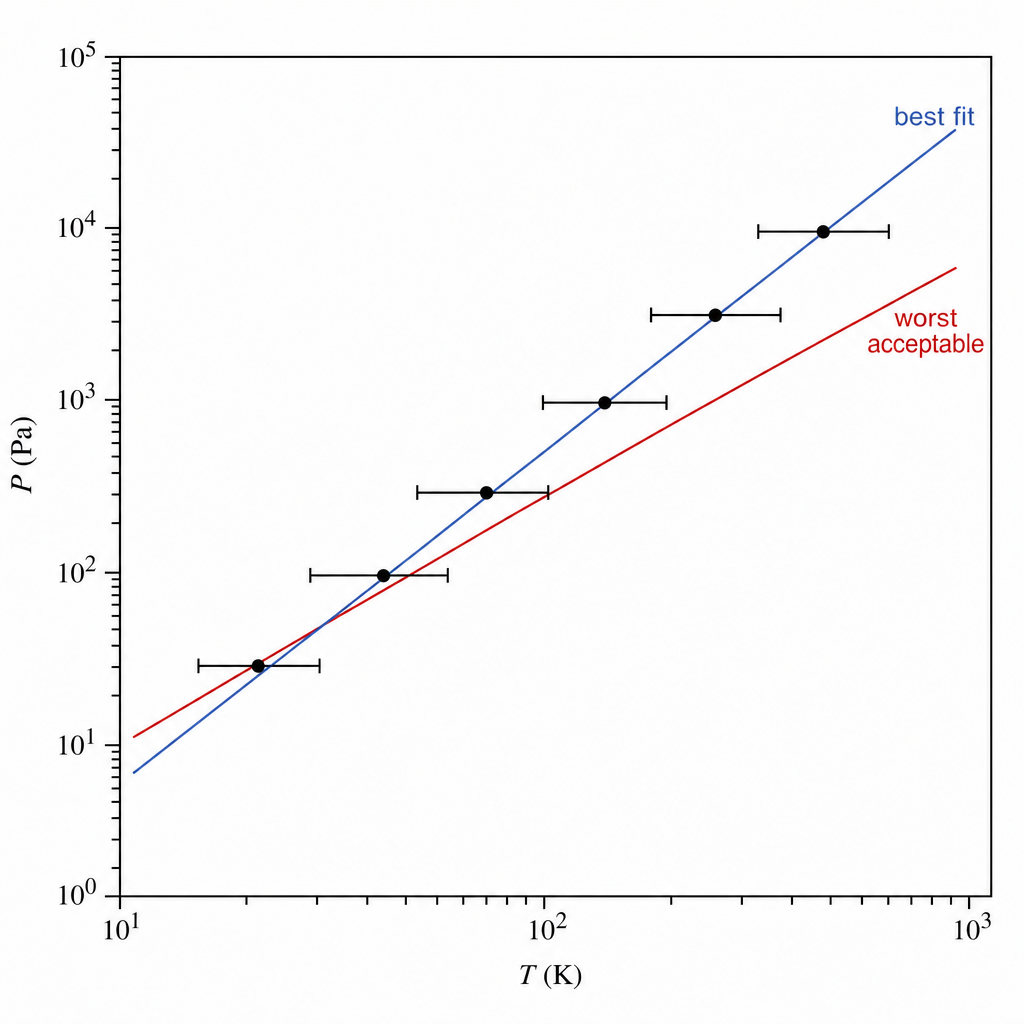
Draw the straight line of best fit and a worst acceptable straight line on your graph. Label both lines.

2M Similar

DifficultyMedium

Worked solution

Draw a straight line of best fit through the plotted points.

Draw a worst acceptable straight line (steepest or shallowest line consistent with all horizontal error bars).

Answer

Both lines drawn and labelled (e.g. “best fit” and “worst acceptable”).

Final answer

Best-fit line and labelled worst acceptable line drawn

Detailed explanation

Background Concept

A best-fit line represents the overall trend of the data. When error bars are present, there is a family of lines that could reasonably fit the data; a “worst acceptable” line is an extreme member of this family (either steepest or shallowest) that still passes through all the error bars.

This is used to estimate uncertainty in the gradient and intercept:

\Delta m \approx |m_{\text{best}}-m_{\text{worst}}|, \qquad \Delta c \approx |c_{\text{best}}-c_{\text{worst}}|.

Understanding the Question

You have already plotted (\lg\lambda) vs (\lg\mu) with horizontal error bars. Now you must:

draw one straight line that best represents the trend,
and another straight line that is still consistent with the error bars but gives an extreme slope.

Approach

Best fit: balance the scatter (roughly equal number of points above and below, not necessarily passing through every point).
Worst acceptable: choose either the steepest or shallowest straight line that can still be considered consistent with the data given the error bars.
Label both lines clearly so you can use them later.

Step-by-Step Reasoning

Draw the best-fit line through the central trend of the points.
For the worst acceptable line, imagine “sliding” a ruler to get the maximum or minimum slope while still intersecting the horizontal error bars of all points (it does not have to go through the central dots; passing through the error bars is enough).

c-ii-best-worst

Key Takeaways

“Worst acceptable” means extreme but still consistent with uncertainties.
Clear labelling prevents confusion when extracting gradients/intercepts.

Common Mistakes

Drawing the worst line through the points rather than through the error bars.
Choosing a line that misses one or more error bars (not acceptable).
Not labelling which line is which.

Things to Be Careful About

With only horizontal error bars, consistency is judged horizontally: your line should pass within the x-range of each bar at the appropriate y-value.
Use a long ruler stroke: extend the line across the full graph to make intercept reading more accurate.

Techniques used

draw a straight line of best fit through scattered datadraw a worst acceptable line consistent with all error barslabel lines clearly for later reading of gradient and intercept

(iii)

Determine the gradient of the line of best fit. Include the absolute uncertainty in your answer.

gradient = ______

2M Similar

DifficultyMedium

Worked solution

Working

Using two points on the best-fit line (widely spaced), e.g.

(x_1,y_1)\approx(0.66,2.70),\qquad (x_2,y_2)\approx(1.26,4.58)

\text{gradient } m = \frac{\Delta y}{\Delta x} = \frac{4.58-2.70}{1.26-0.66} \approx 3.1 \approx 3.2

From worst acceptable line, e.g. (m_{\text{worst}}\approx 3.5).

\Delta m = |m_{\text{best}}-m_{\text{worst}}| \approx |3.2-3.5| = 0.3 \approx 0.4

Answer

(m = 3.2 \pm 0.4)

Final answer

3.2 ± 0.4

Detailed explanation

Background Concept

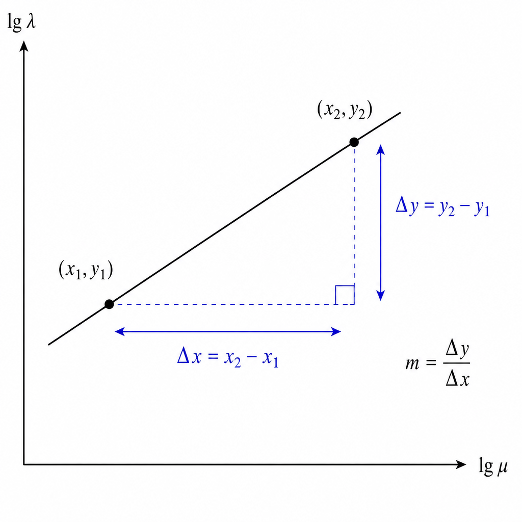
For a straight-line graph, the gradient is

m = \frac{\Delta y}{\Delta x}.

To reduce percentage reading error, you should use two points that are far apart on the drawn line (not necessarily the original data points). When uncertainties are shown by error bars, the uncertainty in the gradient can be estimated by comparing the gradient of the best-fit line with that of a worst acceptable line.

Understanding the Question

You need the gradient of the best-fit line from your log-log plot, and you must give an absolute uncertainty. The uncertainty is found from the difference between the gradients of the best-fit and worst acceptable lines.

Approach

Choose two well-separated points on the best-fit line and calculate (m_{\text{best}}).
Choose two well-separated points on the worst acceptable line and calculate (m_{\text{worst}}).
Take

\Delta m = |m_{\text{best}}-m_{\text{worst}}|.

Step-by-Step Reasoning

Suppose the best-fit line passes near ((0.66,2.70)) and ((1.26,4.58)).

Then

\Delta y = 4.58-2.70 = 1.88,

\Delta x = 1.26-0.66 = 0.60,

m_{\text{best}} = \frac{1.88}{0.60} \approx 3.1 \; (\text{about }3.2).

Repeat the same process for the worst acceptable line, giving an extreme slope (for example around (3.5) for a steeper line).
The absolute uncertainty is the difference:

\Delta m = |3.2-3.5| = 0.3 \approx 0.4.

c-iii-gradient-triangle

Key Takeaways

Use a large triangle on the line to find gradient accurately.
Uncertainty in gradient comes from comparing best and worst acceptable lines.

Common Mistakes

Using two data points instead of two points on the drawn best-fit line (more scatter).
Calculating (\Delta x/\Delta y) instead of (\Delta y/\Delta x).
Quoting uncertainty as half the range without reference to best vs worst line.

Things to Be Careful About

Read coordinates carefully from the axes scales.
Ensure the two points used are far apart (spanning much of the graph width/height) to minimise reading error.
The uncertainty should be absolute (e.g. (\pm 0.4)), not percentage, unless asked.

Techniques used

calculate a gradient using two widely separated points on a straight linedetermine a worst-case gradient from the worst acceptable linecalculate absolute uncertainty as the difference between gradients

(iv)

Determine the $y$ -intercept of the line of best fit. Include the absolute uncertainty in your answer.

$y$ -intercept = ______

2M Similar

DifficultyMedium

Worked solution

Working

Using (y = mx + c) with (m_{\text{best}}\approx 3.2) and a point on the best-fit line, e.g. ((x,y)\approx(0.97,3.66)):

c = y - mx \approx 3.66 - 3.2\times 0.97 \approx 0.59 \approx 0.6

From worst acceptable line, e.g. (c_{\text{worst}}\approx 0.2) or (0.9), so

\Delta c = |c_{\text{best}}-c_{\text{worst}}| \approx 0.4

Answer

(y\text{-intercept } = 0.6 \pm 0.4)

Final answer

0.6 ± 0.4

Detailed explanation

Background Concept

For a straight line

y = mx + c,

the (y)-intercept (c) is the value of (y) when (x=0). On a plotted graph, it can be found by extending the best-fit line to cross the (y)-axis, or calculated using a point ((x,y)) on the line:

c = y - mx.

When uncertainties are present, you compare best-fit and worst acceptable lines to estimate (\Delta c).

Understanding the Question

You must find the (y)-intercept of the best-fit line on the (\lg\lambda) vs (\lg\mu) graph and include an absolute uncertainty using your worst acceptable line.

Approach

Obtain (c_{\text{best}}) by reading intercept directly or using (c=y-mx).
Obtain (c_{\text{worst}}) from the worst acceptable line in the same way.
Take

\Delta c = |c_{\text{best}}-c_{\text{worst}}|.

Step-by-Step Reasoning

If the best-fit gradient is about (m=3.2) and a point on the best-fit line is around ((0.97,3.66)), then

c_{\text{best}} = 3.66 - 3.2\times 0.97 \approx 0.6.

If the worst acceptable line gives a noticeably different intercept (for example around (0.2) or (0.9)), then the difference from the best estimate is around (0.4), so

\Delta c \approx 0.4.

Thus quote (c = 0.6 \pm 0.4).

Key Takeaways

Intercept can be read from the graph or computed from (c=y-mx).
Uncertainty comes from comparing best and worst acceptable lines.

Common Mistakes

Confusing the intercept with (k) (the intercept here is (\lg k), not (k)).
Using a point that is not actually on the best-fit line.
Forgetting to include the uncertainty.

Things to Be Careful About

Extend the drawn line fully to the (y)-axis for a more reliable intercept reading.
Keep consistency: if you use (c=y-mx) for the best line, do the same for the worst line.

Techniques used

read the y-intercept from an extended best-fit linecompute intercept from y = mx + c using a point on the lineestimate intercept uncertainty by comparison with a worst acceptable line

(d)

Using your answers to (a), (c)(iii) and (c)(iv), determine the values of $k$ and $n$ . Include the absolute uncertainties in your values. You need not be concerned with units.

$k$ = ______
$n$ = ______

3M Similar

DifficultyMedium-Hard

Worked solution

From (a):

\lg\lambda = n\lg\mu + \lg k

n = m,\qquad \lg k = c

Using (c)(iii) (m = 3.2 \pm 0.4):

n = 3.2 \pm 0.4

Using (c)(iv) (c = 0.6 \pm 0.4):

k = 10^c = 10^{0.6} \approx 4.0

Uncertainty in (k):

\Delta k \approx k\ln 10\,\Delta c = 4.0\times 2.303\times 0.4 \approx 3.7

Answer

(k = 4.0 \pm 3.7)

(n = 3.2 \pm 0.4)

Final answer

k = 4.0 ± 3.7, n = 3.2 ± 0.4

Detailed explanation

Background Concept

From the linearised relationship

\lg\lambda = n\lg\mu + \lg k,

a plot of (y=\lg\lambda) against (x=\lg\mu) has:

gradient (m = n)
intercept (c = \lg k)

So (k) is found by antilog:

k = 10^c.

If (c) has an uncertainty (\Delta c), then for (k = 10^c):

\frac{\Delta k}{k} \approx \ln 10\,\Delta c

(using differentiation), so

\Delta k \approx k\ln 10\,\Delta c.

Understanding the Question

You have already found the gradient (with uncertainty) and intercept (with uncertainty) from the best-fit line. You must convert these into values of (n) and (k), again with absolute uncertainties.

Approach

Set (n) equal to the best-fit gradient, and (\Delta n) equal to the gradient uncertainty.
Set (c) equal to the intercept (\lg k). Convert to (k) using (10^c).
Convert (\Delta c) into (\Delta k) using

\Delta k \approx k\ln 10\,\Delta c.

Step-by-Step Reasoning

From the graph, suppose

m = 3.2 \pm 0.4, \qquad c = 0.6 \pm 0.4.

Then

n = m = 3.2 \pm 0.4.

Since (c = \lg k),

k = 10^{0.6} \approx 3.98 \approx 4.0.

Uncertainty in (k):

\Delta k \approx k\ln 10\,\Delta c = 4.0\times 2.303\times 0.4 \approx 3.7.

k = 4.0 \pm 3.7.

(Your numbers may differ slightly depending on your exact graph readings; method is what matters.)

Key Takeaways

On a log-log plot: gradient gives the exponent (n), intercept gives (\lg k).
Antilog is needed to get (k).
Uncertainty propagation through (10^c) uses fractional uncertainty (\ln 10,\Delta c).

Common Mistakes

Taking (k=c) instead of (k=10^c).
Using (\Delta k = 10^{\Delta c}) (wrong approach for small uncertainties).
Forgetting to carry the uncertainties into (k) and (n).

Things to Be Careful About

The uncertainty in (k) can be large if (\Delta c) is large; quote an absolute uncertainty as requested.
Keep rounding sensible: do not over-round (c) before taking antilogs, or you can shift (k) noticeably.

Techniques used

use gradient and intercept to identify model constantstake antilogarithms to obtain a constant from its logarithmpropagate uncertainty through an exponential relationship

(e)

The mass of the Sun is $2.0 \times 10^{30}\ \text{kg}$ . The star Alpha Centauri B has a value of $\lambda$ of $0.46$ .

Determine the mass $M$ of Alpha Centauri B.

$M$ = ______ $\text{kg}$

1M Similar

DifficultyMedium

Worked solution

Using (\lambda = k\mu^n) with (\lambda = 0.46), (k\approx 4.0), (n\approx 3.2):

\mu = \left(\frac{\lambda}{k}\right)^{1/n} = \left(\frac{0.46}{4.0}\right)^{1/3.2} \approx 0.51

Mass of Sun (= 2.0\times 10^{30}\ \text{kg}), so

M = \mu(2.0\times 10^{30}) \approx 0.51\times 2.0\times 10^{30} \approx 1.0\times 10^{30}\ \text{kg}

Answer

(M \approx 1.0 \times 10^{30}\ \text{kg})

Final answer

1.0 × 10^30 kg

Detailed explanation

Background Concept

Relative mass is defined as

\mu = \frac{\text{mass of star}}{\text{mass of Sun}}.

So once you have (\mu), the star’s mass is

M = \mu M_{\odot}.

The model relating luminosity and mass is

\lambda = k\mu^n.

To find (\mu), rearrange:

\mu = \left(\frac{\lambda}{k}\right)^{1/n}.

Understanding the Question

You are told:

(M_{\odot} = 2.0\times 10^{30}\ \text{kg})
Alpha Centauri B has (\lambda = 0.46)
From earlier parts you have constants (k) and (n)

You must calculate the mass (M) of Alpha Centauri B.

Approach

Use (\lambda = k\mu^n) to solve for (\mu).
Multiply (\mu) by (M_{\odot}) to get (M) in kg.

Step-by-Step Reasoning

Start with

\lambda = k\mu^n.

Rearrange:

\mu^n = \frac{\lambda}{k}

\mu = \left(\frac{\lambda}{k}\right)^{1/n}.

Substitute (\lambda=0.46), and your values of (k) and (n) (using best estimates, e.g. (k\approx 4.0), (n\approx 3.2)):

\mu = \left(\frac{0.46}{4.0}\right)^{1/3.2} \approx 0.51.

Then convert from relative to actual mass:

M = \mu M_{\odot} \approx 0.51\times 2.0\times 10^{30} \approx 1.0\times 10^{30}\ \text{kg}.

Key Takeaways

Relative quantities convert to absolute quantities by multiplying by the Sun’s value.
Solving a power law often involves raising to the reciprocal power ((1/n)).

Common Mistakes

Using (\mu = (\lambda/k)^n) instead of ((\lambda/k)^{1/n}).
Forgetting to multiply by (2.0\times 10^{30}\ \text{kg}) at the end.
Mixing up (\lambda) and (\mu).

Things to Be Careful About

Use the best-estimate values of (k) and (n) (not their logarithms).
Give the final mass in kg and in standard form, matching the significant figures implied by the data (typically 2 s.f. here).

Techniques used

rearrange a power law to solve for the mass ratiosubstitute into the model to calculate an unknown quantityconvert from relative mass to actual mass

Physics 9702/54 — May/June 2025

Variables

Diagram / arrangement

Procedure and measurements

Analysis (to find PPP and QQQ)

Safety

Background Concept

Understanding the Question

Approach

Step-by-Step Reasoning

(1) Setting the geometry and keeping zzz constant

(2) Making vvv known and constant

(3) Measuring ddd reliably

(4) Linear graph and extracting PPP and QQQ

Key Takeaways

Common Mistakes

Things to Be Careful About

Answer

Background Concept

Understanding the Question

Approach

Step-by-Step Reasoning

Key Takeaways

Common Mistakes

Things to Be Careful About

Background Concept

Understanding the Question

Approach

Step-by-Step Reasoning

Key Takeaways

Common Mistakes

Things to Be Careful About

Answer

Background Concept

Understanding the Question

Approach

Step-by-Step Reasoning

Key Takeaways

Common Mistakes

Things to Be Careful About

Answer

Background Concept

Understanding the Question

Approach

Step-by-Step Reasoning

Key Takeaways

Common Mistakes

Things to Be Careful About

Working

Answer

Background Concept

Understanding the Question

Approach

Step-by-Step Reasoning

Key Takeaways

Common Mistakes

Things to Be Careful About

Working

Answer

Background Concept

Understanding the Question

Approach

Step-by-Step Reasoning

Key Takeaways

Common Mistakes

Things to Be Careful About

Answer

Background Concept

Understanding the Question

Approach

Step-by-Step Reasoning

Key Takeaways

Common Mistakes

Things to Be Careful About

Answer

Background Concept

Understanding the Question

Approach

Step-by-Step Reasoning

Key Takeaways

Analysis (to find $P$ and $Q$ )

(1) Setting the geometry and keeping $z$ constant

(2) Making $v$ known and constant

(3) Measuring $d$ reliably

(4) Linear graph and extracting $P$ and $Q$