Physics 9702/52 — May/June 2025
Cambridge A-Level · Planning, Analysis and Evaluation · worked solutions for every part, with the mark scheme
Topics Analysis, Conclusions and Evaluation · Planning
A thin solid disc of radius and thickness is attached to a thin axle. String is wrapped around the axle, as shown in Fig. 1.1.
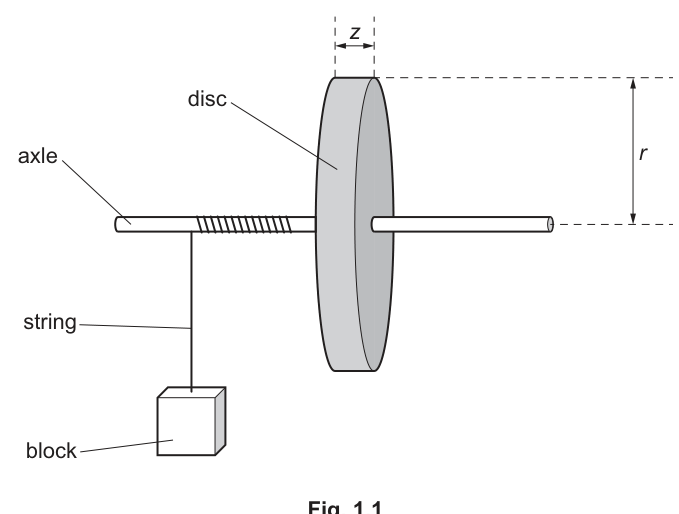
A block of mass is attached to the string.
The block is released from rest and falls downwards. The block has speed when it has fallen through a distance from the point of release. The value of is determined using one light gate connected to a timer.
It is suggested that is related to by the relationship
where and are constants.
Plan a laboratory experiment to test the relationship between and .
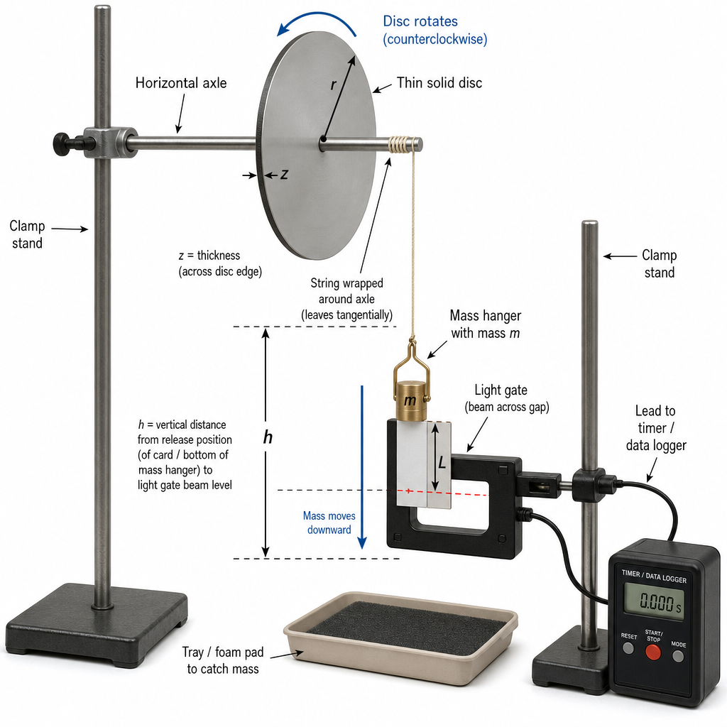
Draw a diagram showing the arrangement of your equipment.
Explain how the results could be used to determine values for and .
In your plan you should include:
- the procedure to be followed
- the measurements to be taken
- the control of variables
- the analysis of the data
- any safety precautions to be taken.
Apparatus
Disc + axle on low-friction bearings, string, mass hanger + slotted masses, light gate + timer/data logger, card/flag of known length , metre rule, clamp stand(s), vernier calipers / micrometer screw gauge (for and ).
Variables
- Independent: (total hanging mass).
- Dependent: after falling distance .
- Controlled: (fixed), same disc/axle (so and constant), same string and wrapping (no slip), release from rest each run, light gate position fixed, card length fixed.
Procedure and measurements
- Measure disc radius (e.g. diameter with vernier calipers then halve) and thickness (micrometer). Record uncertainties.
- Attach a card/flag of measured length to the falling mass so it will pass through the light gate.
- Wrap string around axle, attach mass , and set the light gate a vertical distance below the release point (measure with a metre rule).
- Release the mass from rest without pushing. Record the time for which the light gate beam is interrupted by the flag.
- Calculate the speed at the gate:
- Repeat at least 3 times for the same and average (or ).
- Change by adding slotted masses; use at least 6 different values spanning a suitable range; repeat steps 3–6.
Analysis of data (test of relationship)
For each :
- compute and then
- compute .
Given
let
so
Plot a graph of (y-axis) against (x-axis). A straight line supports the relationship.
Determination of and
From the graph:
- intercept , hence
- gradient , hence
(using measured and calculated ).
Safety
Clamp the apparatus securely; keep feet/hands clear of falling masses; use a tray/soft landing pad to catch the mass; ensure the string cannot whip loose and that the stand cannot topple.
See working
Background Concept
The falling mass loses gravitational potential energy and causes the disc to rotate via the string on the axle. The measured quantity in this experiment is the instantaneous speed of the mass after it has fallen through a fixed vertical distance .
The question provides a model that predicts a linear relationship:
where and are constants for this system, and and are properties of the disc.
A standard way to “test a relationship” in Paper 5 is:
- rearrange into the straight-line form ,
- choose what to plot so that the data should lie on a straight line,
- use the gradient and intercept to calculate the constants.
A single light gate can measure an instantaneous speed if a card/flag of known length passes through it. If the light beam is blocked for time , then the speed at the gate is
provided the speed does not change much while the card passes through (using a short card helps).
Understanding the Question
You must plan an experiment where you vary the mass and measure the speed after the mass has fallen the same distance each time. You must use only one light gate, so the typical method is a single interrupt card.
You are also asked to explain how your results can be used to find numerical values of and . That means your analysis must produce both a gradient and an intercept (two pieces of information) so you can solve for two unknown constants.
The disc geometry and appear in the equation, so you must measure them (or they must be known). In a real lab, you measure them with calipers/micrometer.
Approach
- Choose a fixed position of the light gate, a distance below the release point.
- For each chosen mass , release from rest and use the light gate to obtain at that position.
- Process each run into the variables that appear in the linear form: compute and .
- Plot against so the relationship becomes .
- Read gradient and intercept and then calculate:
- from the intercept ,
- from the gradient .
- Control variables so that only changes, and include safety measures for a falling mass.
Step-by-Step Reasoning
1) Set-up and measurements
- Mount the disc/axle so it can rotate freely (minimise bearing friction).
- Wrap the string neatly around the axle so it does not overlap; attach the mass hanger.
- Measure the flag length with a ruler (small uncertainty; ensure it is rigid and does not bend).
- Fix the light gate on a clamp stand.
- Define the release point (e.g. bottom of the mass hanger level with a marked reference line) and measure down to the light gate beam with a metre rule.
- Measure (best: measure diameter at several orientations with vernier calipers and average, then halve) and measure thickness with a micrometer.
2) Collecting data for one mass
For a chosen total mass :
- Raise the mass so the card will pass through the light gate after falling distance .
- Release without pushing (so initial speed is as close to zero as possible).
- The timer gives the interrupt time .
- Calculate
- Repeat several times and average (or average ). Repeats reduce random error from release technique and any wobble.
3) Varying the independent variable
Change by adding slotted masses. Take at least 6 values over a good range so your graph has a reliable gradient and intercept.
4) Linearisation and graph
Start from:
Recognise that the only term involving is . So define:
Then the equation becomes:
So plotting against should give a straight line.
5) Extracting and
From the straight line:
- Intercept equals , so
- Gradient equals . Rearranging gives
You can only do this if you have already found from the intercept.
(If you include uncertainties, you would estimate uncertainties in and using worst acceptable lines, then propagate those into and .)
6) Control of variables (why it matters)
To make the test fair, only should change:
- Keep the same by keeping the light gate fixed and using the same release reference point.
- Use the same disc and axle (so and are fixed).
- Keep the string and wrapping method the same: slipping changes the relationship between translational motion and rotation.
- Keep the flag the same length and in the same orientation through the gate.
7) Safety
The main risk is a falling mass and toppling equipment:
- Clamp stands firmly and consider adding a heavy base.
- Use a tray/box or foam pad to catch the mass.
- Keep hands/feet clear of the drop zone.
- Ensure the string cannot fly off sideways.
Key Takeaways
- A single light gate can measure instantaneous speed using a flag of known length: .
- Linearising an equation into is the most direct way to test a relationship and obtain constants.
- Plotting against provides both an intercept (to find ) and a gradient (to find ).
- Good planning requires clear variable control, repeats, and safe/secure apparatus.
Common Mistakes
- Plotting the wrong variables (e.g. vs ) so the line is not linear and gradient/intercept do not match the model.
- Forgetting that only one light gate is allowed and attempting a two-gate speed method.
- Not measuring/mentioning and even though they are needed to compute .
- Changing unintentionally by releasing from different starting points for different masses.
- Using too few values of (insufficient data to justify a straight line and reliable gradient/intercept).
Things to Be Careful About
- Ensure the card length is measured along the direction of motion through the gate.
- Use a short flag so the speed does not change much while it passes the beam.
- Release from rest consistently; do not push the mass.
- Make sure the string does not slip on the axle and does not overlap between turns.
- Use a sensible mass range: very small may not overcome friction reliably; very large may cause unsafe speeds or slipping.
A student investigates a circuit containing capacitors. The circuit is connected with a capacitor of capacitance , as shown in Fig. 2.1.
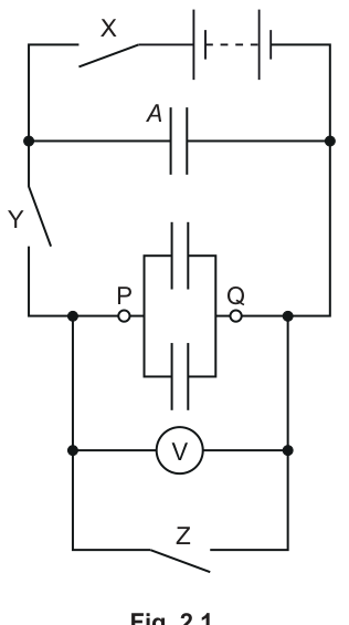
Two capacitors, each of capacitance , are connected in parallel between P and Q.
Initially, switch X and switch Z are closed and switch Y is open.
Switches X and Z are opened. Switch Y is then closed. The maximum potential difference between P and Q is measured using the voltmeter. This procedure is repeated and the mean maximum potential difference between P and Q is determined.
The experiment is then repeated by changing the number of capacitors, each of capacitance , connected in parallel between P and Q.
It is suggested that and are related by the equation
where is the electromotive force (e.m.f.) of the battery.
A graph is plotted of on the -axis against on the -axis.
Determine expressions for the gradient and -intercept.
gradient = ______
-intercept = ______
From
So
gradient = C/(EA); y-intercept = 1/E
Background Concept
To test a proposed relationship experimentally, we often rearrange it into a straight-line form
where is the gradient and is the y-intercept. Plotting the correct variables then allows constants in the original equation to be found from and .
Understanding the Question
You are told the suggested relationship is
and a graph is plotted of (y-axis) against (x-axis). The task is to rearrange the equation so that is expressed as a linear function of , then read off the gradient and y-intercept.
Approach
- Make the subject.
- Take the reciprocal to obtain .
- Expand into “(constant) + (constant)” so it matches .
Step-by-Step Reasoning
Starting with
divide both sides by :
Now take the reciprocal:
Split the numerator into two terms:
Comparing with where and :
- gradient
- intercept (because cancels)
Key Takeaways
- Linearise by rearranging into .
- For a vs plot, the coefficient of is the gradient, and the remaining constant term is the intercept.
Common Mistakes
- Stopping at and not converting to .
- Giving intercept as but not recognising it simplifies to .
- Mixing up which variable is on which axis (here , ).
Things to Be Careful About
- is dimensionless, so the gradient has units of .
- Keep algebra exact; simplifications like can make later parts much easier.
Values of and the two measured values of the maximum potential difference and are given in Table 2.1.
Table 2.1
| 2 | 4.30 | 4.20 | ||
| 3 | 3.65 | 3.75 | ||
| 4 | 3.30 | 3.20 | ||
| 5 | 2.85 | 2.95 | ||
| 6 | 2.65 | 2.55 | ||
| 7 | 2.30 | 2.40 |
Calculate and record values of and in Table 2.1. Include the absolute uncertainties in and .
For each row:
Completed values (with absolute uncertainties):
| 2 | ||||
| 3 | ||||
| 4 | ||||
| 5 | ||||
| 6 | ||||
| 7 |
See completed table in working
Background Concept
When a quantity is measured more than once, a common estimate of the absolute uncertainty from repeats is half the range:
If you then calculate a derived quantity, you must propagate uncertainty. For a reciprocal,
the approximate absolute uncertainty is found using differentiation:
Understanding the Question
You are given two readings and for each . You must:
- Find the mean maximum p.d. .
- Find .
- Include absolute uncertainties in both and in the table.
Approach
- Compute the mean: .
- Use half-range for uncertainty in .
- Compute .
- Propagate uncertainty for the reciprocal using .
Step-by-Step Reasoning
Example for :
Mean:
Uncertainty in (half range):
Reciprocal:
Uncertainty in reciprocal:
Repeat the same steps for all .
Key Takeaways
- Mean from repeats: .
- Repeat uncertainty estimate: half the range.
- Reciprocal uncertainty: .
Common Mistakes
- Using the full range instead of half the range for .
- Calculating percentage uncertainty when the question asks for absolute uncertainty.
- Forgetting units for (it is ).
- Rounding too aggressively so the plotted points lose precision.
Things to Be Careful About
- Keep consistent decimal places within a column.
- Uncertainties should usually be to 1 (or sometimes 2) significant figures, and the quoted value should match that precision.
- Use the mean in , not one of the individual readings.
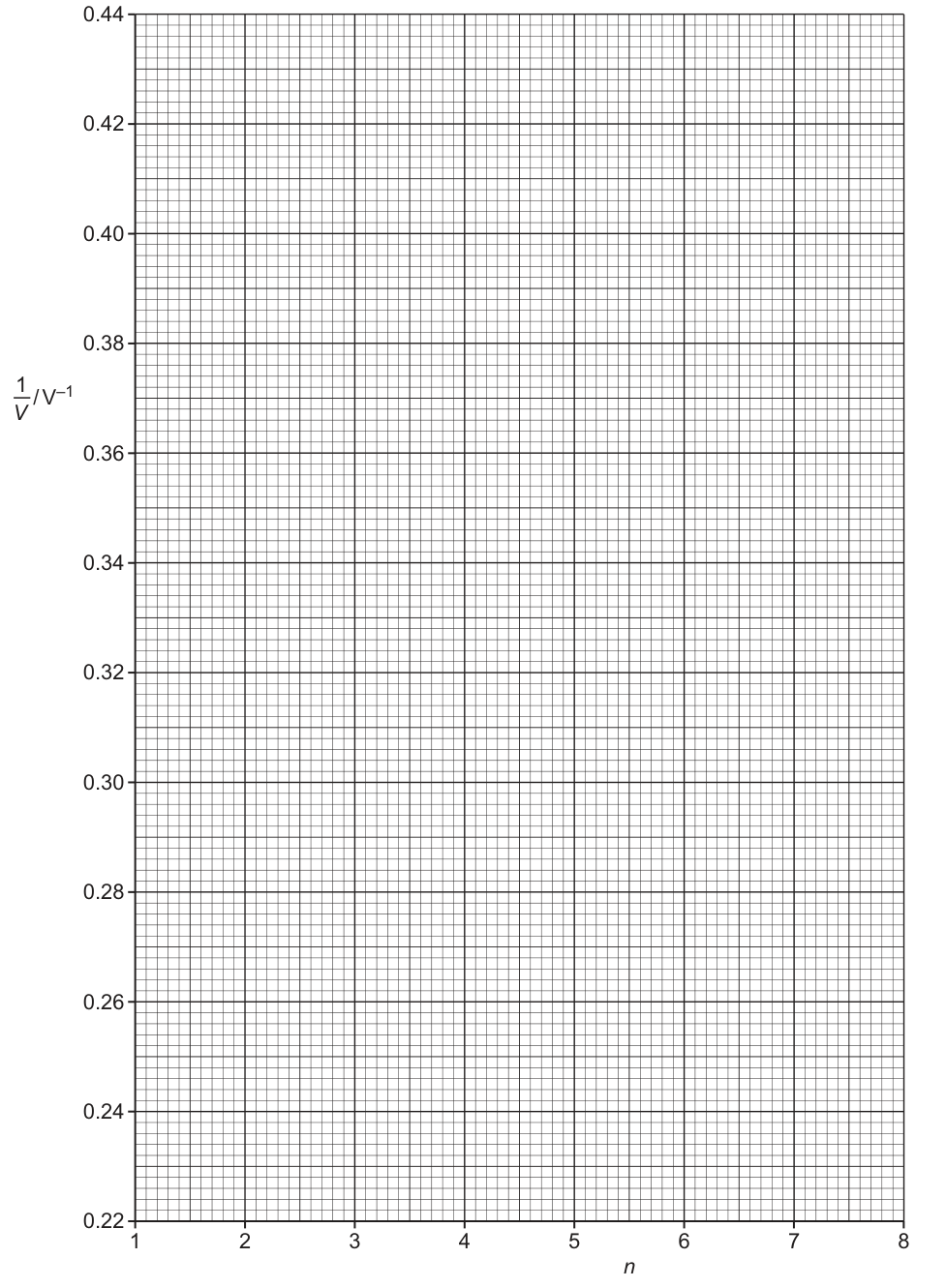
Plot the points from Table 2.1 and draw vertical error bars of size for each point.
See plotted graph with error bars
Background Concept
A graph is used to test a linear relationship and to extract constants from its gradient and intercept. Error bars show the uncertainty in measured (or derived) values; here only has uncertainty bars because is exact.
Understanding the Question
You must plot on the y-axis against on the x-axis, using your calculated values, and include error bars for using the absolute uncertainties you found in part (b).
Approach
- Label axes with quantity and unit: (no unit) and .
- Plot each point accurately.
- For each point, draw a vertical error bar from to .
Step-by-Step Reasoning
- Choose a scale that uses at least half of the provided grid in both directions.
- Plot the six points (for to ) at their calculated y-values.
- For each plotted point, use your uncertainty to mark the top and bottom of the error bar in y.
- Draw neat, centred error bars (usually with small horizontal end-caps).
Key Takeaways
- Error bars represent the uncertainty range for the plotted quantity.
- Here, is a count, so it is treated as exact (no x-error bars).
Common Mistakes
- Omitting units in the axis label for .
- Drawing error bars of the wrong size (e.g. using instead of ).
- Plotting instead of .
Things to Be Careful About
- Plotting precision: use at least half a small square when reading positions.
- Ensure error bars are vertical (since they apply to only).
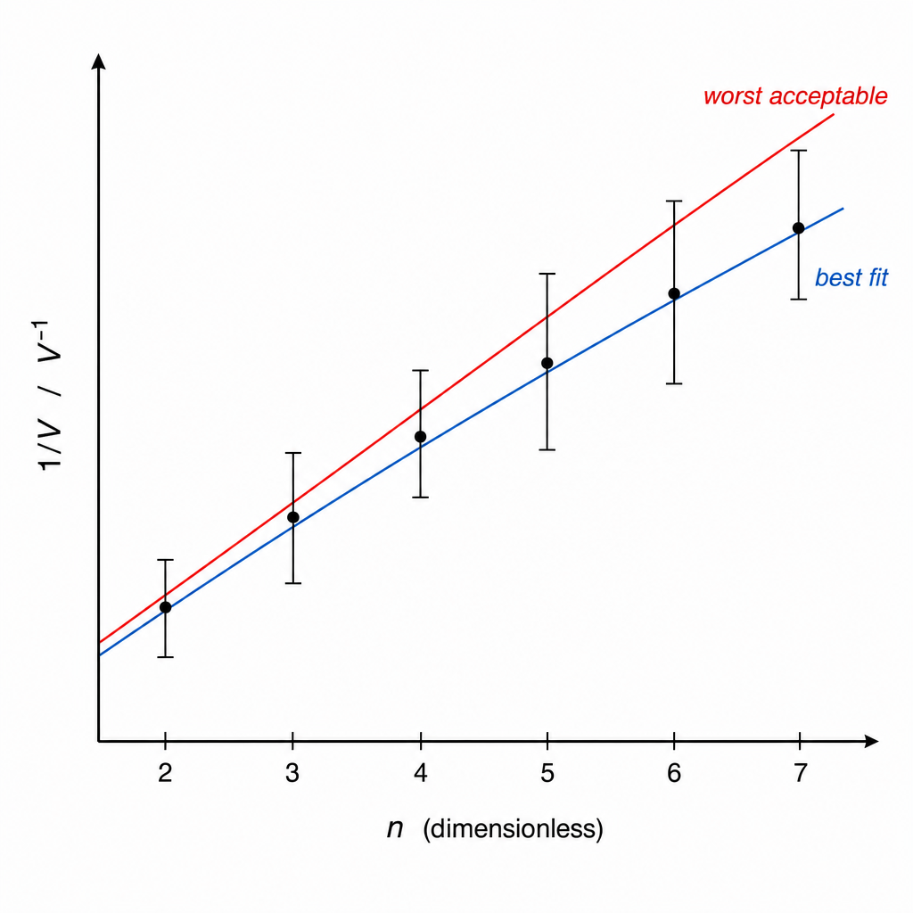
Draw the straight line of best fit and a worst acceptable straight line on your graph. Label both lines.
Draw a straight line of best fit through the plotted points.
Draw a worst acceptable straight line (steepest or shallowest) that still passes through all the error bars.
Label the two lines clearly (e.g. “best fit” and “worst acceptable”).
See labelled best-fit and worst-acceptable lines
Background Concept
A line of best fit represents the overall trend of the data (balancing points above and below). A worst acceptable line is drawn to estimate uncertainty in gradient/intercept: it is the steepest or shallowest line that is still consistent with the data within their error bars.
Understanding the Question
You have already plotted points of vs with vertical error bars. Now you must add:
- one best-fit straight line,
- one worst acceptable straight line,
and label them.
Approach
- Best-fit line: aim for roughly equal scatter about the line across the whole range.
- Worst acceptable line: pivot to make it as steep (or as shallow) as possible while still intersecting every vertical error bar somewhere.
- Label both; this is essential so the examiner knows which line you used for each calculation.
Step-by-Step Reasoning
- Use a ruler to draw one straight line that represents the trend: do not join dot-to-dot.
- Check visually that the line passes near the middle of the error bars overall.
- Draw a second line:
- try the steepest possible line that still crosses all error bars,
- and/or the shallowest possible line that still crosses all error bars.
- Choose the line (steepest or shallowest) that gives the largest difference in gradient (and/or intercept) compared with your best-fit line; this is typically used in the next parts.
- Write labels directly on the graph near each line.
Key Takeaways
- Worst acceptable line is an uncertainty tool, not a “second best-fit”.
- It must be consistent with the error bars, not necessarily with the central points.
Common Mistakes
- Drawing the worst line through the plotted points rather than through the error bars.
- Drawing a line that misses one or more error bars (then it is not acceptable).
- Forgetting to label which line is which.
Things to Be Careful About
- Use the full span of the graph when judging acceptability.
- Keep the lines straight and drawn with a ruler; small wobbles can change gradient readings.
Determine the gradient of the line of best fit. Include the absolute uncertainty in your answer.
gradient = ______
Working
Using a large triangle on the best-fit line,
Worst acceptable gradient gives
Answer
(3.80 ± 0.24) × 10^-2 V^-1
Background Concept
For a straight-line graph of against , the gradient is
To reduce percentage reading error, you should use a large triangle (points far apart on the line).
To estimate the uncertainty in gradient with error bars, Paper 5 typically uses a “best line” and a “worst acceptable line”. A common method is:
where is the steepest or shallowest acceptable line (whichever is further from ).
Understanding the Question
You must find the gradient of the best-fit line on your vs graph, and include an absolute uncertainty based on your worst acceptable line.
Approach
- Choose two widely separated points on the best-fit line (not necessarily the plotted data points).
- Calculate .
- Repeat using the worst acceptable line to get .
- Take the absolute difference to get the uncertainty.
Step-by-Step Reasoning
- Because is dimensionless, the unit of gradient is simply the unit of , i.e. .
- Using widely spaced points keeps fractional reading uncertainty low.
- The worst acceptable line is constrained by the error bars; it represents an extreme but still plausible gradient.
A representative set of values gives:
and a worst acceptable gradient around
so
Key Takeaways
- Use a large triangle for the gradient.
- Uncertainty in gradient comes from comparing best and worst acceptable lines.
Common Mistakes
- Using instead of .
- Using two points very close together, giving a poor gradient.
- Taking half the difference between gradients when the scheme expects .
Things to Be Careful About
- Read values from the line, not from the individual plotted points.
- Quote the gradient to a sensible number of significant figures consistent with the graph precision.
Determine the -intercept of the line of best fit. Include the absolute uncertainty in your answer.
-intercept = ______
Working
From the best-fit line,
From the worst acceptable line,
Answer
(0.157 ± 0.010) V^-1
Background Concept
In
is the y-intercept, i.e. the value of when . On a graph, it is where the line crosses the y-axis.
The uncertainty in is found by comparing the intercept from the best-fit line with the intercept from the worst acceptable line:
Understanding the Question
You must determine the y-intercept of your best-fit line on the vs graph, and give an absolute uncertainty using the worst acceptable line.
Approach
- Extend the best-fit line to the y-axis () and read off .
- Do the same for the worst acceptable line to get .
- Take the absolute difference.
Step-by-Step Reasoning
- Since the y-axis is , the intercept has units .
- Even though your data starts at , you can still find the intercept by extending the straight line to .
A representative reading gives
and a worst acceptable intercept around
so
Key Takeaways
- The intercept is read at by extending the straight line.
- Use the worst acceptable line to estimate an intercept uncertainty.
Common Mistakes
- Reading the intercept at instead of at .
- Forgetting to extend the line accurately to the axis.
- Quoting an intercept uncertainty that is unrealistically small compared with the graph scale.
Things to Be Careful About
- Use the same method for both best and worst lines.
- Ensure your uncertainty is an absolute uncertainty (not a percentage here).
Using your answers to (a), (c)(iii) and (c)(iv), determine the values of and . Include appropriate units.
Data:
= ______
= ______
From (a):
So y-intercept :
Gradient , hence
Using , , :
Answer
E = 6.37 V, C = 0.53 mF
Background Concept
Once a relationship has been linearised to
the graph directly gives (gradient) and (intercept). By comparing this with the theoretical rearrangement, you can solve for the physical constants.
Understanding the Question
You have already found in (a) that
You also determined from the graph:
- best-fit gradient (with units ),
- best-fit intercept (with units ).
You are given and must calculate and .
Approach
- Use the intercept: since , invert it to get .
- Use the gradient: , rearrange to .
- Substitute so that you only need , , and .
Step-by-Step Reasoning
From
identify
So if ,
Now use
and substitute :
Putting in mF will give in mF (since is dimensionless):
Key Takeaways
- Intercept gives directly here because it simplifies to .
- Gradient together with and gives .
- Always carry units through to confirm the result makes sense.
Common Mistakes
- Using but forgetting it simplifies, then making algebra errors.
- Mixing up gradient and intercept when substituting.
- Converting to farads but leaving in mF without stating units clearly.
Things to Be Careful About
- is in , so is in V.
- has no unit, so both gradient and intercept have the same unit .
- Use the best-fit values (not the worst-line values) for the central estimates of and .
Determine the percentage uncertainty in your value of .
percentage uncertainty = ______
Using
Answer
22%
Background Concept
For multiplication and division, fractional uncertainties add:
- If , then .
- If , then .
This is the standard Paper 5 method for percentage uncertainty.
Understanding the Question
You found using (gradient), (intercept), and . You are asked for the percentage uncertainty in , so you must combine the uncertainties in these inputs.
Approach
- Use the expression you used to calculate :
- Add fractional uncertainties from , , and .
- Multiply by to convert to a percentage.
Step-by-Step Reasoning
Start from
So
- gives .
- and come from your best-fit vs worst acceptable line method.
Add the three contributions and convert to a percentage.
Key Takeaways
- Always pick the correct form of before combining uncertainties.
- For products/quotients, add fractional uncertainties.
Common Mistakes
- Subtracting fractional uncertainties because one quantity is in the denominator (you still add them).
- Using percentage uncertainty in but absolute uncertainty in (must be consistent: fractional then convert).
- Forgetting to multiply by .
Things to Be Careful About
- Use the absolute uncertainties you actually obtained from the graph.
- Quote the final percentage uncertainty to a sensible whole number (typically).
The experiment is repeated with 10 capacitors, each of capacitance , connected in parallel between P and Q. Determine the maximum potential difference between P and Q.
= ______
Using
with , , , :
Answer
1.9 V
Background Concept
Once you have determined the constants in an empirical/theoretical relationship, you can use the relationship to predict the dependent variable for new values of the independent variable.
Here the model is
so for a given you can calculate .
Understanding the Question
The experiment is repeated with capacitors in parallel. Using your calculated values of and (and given ), you must predict the maximum potential difference between P and Q.
Approach
Rearrange to make the subject:
Then substitute and your values for , , and .
Step-by-Step Reasoning
- Start from
- Divide by :
-
Substitute values. If you keep and both in mF, the mF cancels in numerator/denominator, giving volts as required.
-
Evaluate and round sensibly (typically to 2 s.f. for a 1-mark numerical answer).
Key Takeaways
- Use the derived relationship to extrapolate/interpolate to a new .
- Keep capacitances in consistent units so they cancel cleanly.
Common Mistakes
- Substituting into the graph equation for but forgetting to invert to get .
- Mixing units (e.g. putting in F and in mF).
- Arithmetic error in the denominator .
Things to Be Careful About
- must be evaluated before dividing.
- Quote with unit V and appropriate significant figures.