Physics 9702/51 — May/June 2025
Cambridge A-Level · Planning, Analysis and Evaluation · worked solutions for every part, with the mark scheme
Topics Analysis, Conclusions and Evaluation · Planning
Fig. 1.1 shows a thin coil of cross-sectional area and length connected to a resistor of resistance and two terminals.
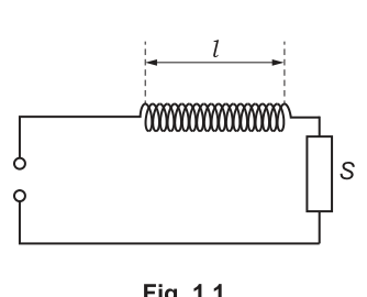
An alternating voltage is applied to the terminals. The peak value of the alternating voltage is and the frequency is . The peak value of the potential difference across the resistor is determined using an oscilloscope.
It is suggested that is related to by the relationship
where is the number of turns on the coil and is a constant.
Plan a laboratory experiment to test the relationship between and .
Draw a diagram showing the arrangement of your equipment.
Explain how the results could be used to determine a value for .
In your plan you should include:
- the procedure to be followed
- the measurements to be taken
- the control of variables
- the analysis of the data
- any safety precautions to be taken.
Answer
Variables
- Independent variable: frequency of the applied a.c. signal.
- Dependent variable: peak p.d. across resistor .
- Control variables: peak applied voltage (keep constant), resistor , coil geometry (, ) and number of turns (same coil), temperature (to keep resistances constant).
Apparatus
Signal generator, thin coil (air-cored), known resistor (and DMM to check ), dual-channel oscilloscope, connecting leads, metre rule, vernier calipers/micrometer.
Procedure and measurements
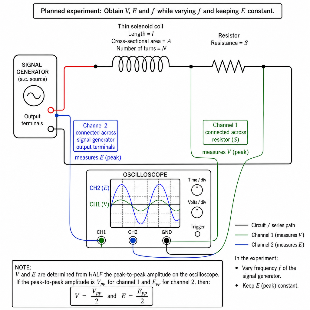
- Connect coil in series with resistor to the signal generator.
- Connect oscilloscope channel 1 across the resistor to measure peak p.d. .
- Connect oscilloscope channel 2 across the signal generator output (terminals) to measure peak applied voltage .
- Set the signal generator to a sinusoid. Choose a value of (e.g. a few volts peak) and keep it constant for all readings (monitor channel 2 and adjust amplitude if necessary).
- Vary over a suitable range with at least 6 values.
- For each , measure:
- from the signal generator display or from the oscilloscope period (),
- from the oscilloscope trace (measure and use ),
- similarly (or confirm it remains constant).
Repeat readings and average.
- Measure coil dimensions once: measure coil diameter with calipers and calculate ; measure coil length with a ruler. Determine/record (from coil specification or by counting turns).
Analysis of data (test of relationship and finding )
Rearrange
Calculate for each and plot a graph of (vertical) against (horizontal).
- Expect a straight line through the origin.
- Gradient is
so
Safety
- Use low-voltage a.c. output from the signal generator.
- Use a resistor with adequate power rating; switch off if resistor/coil heats up.
- Avoid short circuits and exposed conductors; keep leads tidy.
- Take care with oscilloscope earth reference (ensure the generator output is not inadvertently shorted to ground).
See working
Background Concept
A coil has inductance, so with an alternating current it produces a back e.m.f. that depends on how quickly the current changes. In an a.c. circuit with a coil in series with a resistor, the current (and therefore the resistor p.d.) depends on frequency. The question provides a suggested relationship:
Here:
- is the peak applied voltage (across the supply terminals),
- is the peak p.d. across the resistor ,
- is the coil cross-sectional area,
- is the coil length,
- is number of turns,
- is a constant to be determined experimentally.
The important experimental skill is to turn this into a linear form so you can test it with a straight-line graph and use the gradient to find .
Understanding the Question
You are given a series circuit (coil + resistor) driven by an a.c. source. You can vary the frequency and you can measure the peak resistor voltage using an oscilloscope. You must:
- design a method to take readings of for different while keeping other quantities controlled,
- show how to process the readings to test whether the proposed proportionality is correct,
- explain clearly how is obtained from your graph.
Because the relationship involves and , you either need to measure as well or keep constant and known. Similarly, , , , and must be known/constant.
Approach
- Choose variables: vary (independent variable) and measure (dependent variable).
- Control key factors: keep constant because it appears in the equation; keep the same resistor and the same coil so , , remain constant.
- Collect data carefully: for each , read peak values from the oscilloscope (use peak-to-peak then halve).
- Linearise: compute and plot it against so that the graph should be a straight line.
- Extract from gradient: use the gradient relationship to calculate .
Step-by-Step Reasoning
-
Circuit and measurements
- Put the coil and resistor in series with a signal generator.
- Use oscilloscope channel 1 across the resistor to measure .
- Use oscilloscope channel 2 across the generator output to measure (this is also a good check that is being kept constant).
-
Choosing the frequency range and number of readings
- Pick at least 6 different frequencies spanning a wide range (enough to show a clear trend and allow a best-fit line).
- Ensure the waveforms remain sinusoidal and the oscilloscope trace is stable.
-
Keeping constant (control of variables)
- When you change , the generator amplitude may drift. The relationship is only being tested properly if is constant.
- Monitor on channel 2; after each frequency change, adjust the generator amplitude so that the peak (or peak-to-peak) value is the same as your chosen value.
-
Reading peak values from the oscilloscope
- Measure peak-to-peak voltage from the number of vertical divisions multiplied by the volts-per-division.
- Convert to peak using
- Repeat the measurement at each frequency and average to reduce random reading error.
-
Measuring coil parameters
- Measure the coil diameter with vernier calipers (take several readings around the coil and average).
- Calculate area
- Measure coil length with a ruler (or calipers if short).
- Record (count turns or use manufacturer’s stated value).
-
Data processing and graph
- For each frequency, calculate
- Plot (vertical axis) against (horizontal axis).
- If the suggested relationship is correct, the graph should be a straight line with (approximately) zero intercept because it predicts direct proportionality.
-
Determining from the gradient
- From the gradient of the vs graph is
- Hence
-
Uncertainties (good practice in Paper 5 plans)
- State likely dominant uncertainties: reading oscilloscope amplitudes, keeping constant, measurement of (affects ), and .
- To estimate uncertainty in , you can use the uncertainty in the gradient (from a worst acceptable line) and combine with percentage uncertainties in , , and (if is not exact).
Key Takeaways
- A planning question is scored for: clear variables, workable method, correct measurements, control of variables, and a graph/analysis that directly tests the proposed equation.
- Linearisation is crucial: plotting against makes the test “straight line through origin” and gives a clean route to via the gradient.
- Measuring peak quantities on an oscilloscope is typically done via peak-to-peak then halving.
Common Mistakes
- Varying frequency but not keeping constant (then changes in are not solely due to ).
- Plotting the wrong graph (e.g. vs ) without using the provided linear form.
- Using RMS values for one voltage and peak values for the other (mixing definitions).
- Forgetting to state how and are measured, or not stating how is known.
- Not stating how to obtain from the graph (must link gradient to explicitly).
Things to Be Careful About
- Oscilloscope readings: always convert divisions correctly and be consistent about peak vs peak-to-peak.
- The oscilloscope ground clip can create a short if connected incorrectly; ensure the generator and oscilloscope grounds are compatible.
- Heating: if current is too large, (and coil resistance) may change with temperature, affecting . Use modest voltages and allow cooling time if needed.
- Graph quality: use a wide frequency range, enough points, and a best-fit line; if discussing uncertainty, mention worst acceptable line for the gradient uncertainty.
A student investigates an electrical circuit.
The circuit is set up as shown in Fig. 2.1.
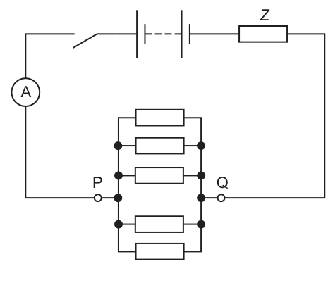
A battery of negligible internal resistance is connected to a resistor of resistance . Five resistors, each of resistance , are connected in parallel between P and Q.
The switch is closed. The total current in the circuit is measured using the ammeter.
The experiment is then repeated by changing the number of resistors, each of resistance , connected in parallel between P and Q.
It is suggested that and are related by the equation
where is the electromotive force (e.m.f.) of the battery.
A graph is plotted of on the -axis against on the -axis.
Determine expressions for the gradient and -intercept.
gradient = ______
-intercept = ______
From
Answer
Gradient
-intercept
Gradient = R/E, y-intercept = Z/E
Background Concept
A straight-line graph has the form
where is the gradient and is the -intercept. In many experiments, you are given a physical relationship that is not obviously in this form, so you rearrange it until the plotted variables match and .
For resistors in parallel, the equivalent resistance is reduced. For identical resistors each of resistance in parallel,
Understanding the Question
The circuit has a fixed series resistor and a variable parallel combination between and . The suggested relationship is
You are told to plot (vertical axis) against (horizontal axis). So we want an equation with on the left and appearing linearly on the right.
Approach
- Divide the given equation by to make .
- Expand the brackets so it looks like (constant), + (constant).
- Compare with to read off gradient and intercept.
Step-by-Step Reasoning
Start with
Divide both sides by :
Split the bracketed term:
Now match to with and .
So:
- gradient
- intercept .
Key Takeaways
- Linearise by rearranging into .
- The coefficient of the plotted variable is the gradient.
- The constant term is the -intercept.
Common Mistakes
- Leaving the equation as and trying to read gradient directly.
- Using instead of when matching to the graph axes.
- Mixing up which constant is gradient and which is intercept.
Things to Be Careful About
- Ensure the plotted variables exactly match the rearranged equation: here it must be vs .
- Keep outside the bracket correctly when dividing through: both terms must be divided by .
Values of , and are given in Table 2.1.
Table 2.1
| 5 | 0.200 | ||
| 6 | 0.167 | ||
| 7 | 0.143 | ||
| 8 | 0.125 | ||
| 9 | 0.111 | ||
| 11 | 0.0909 |
Calculate and record values of in Table 2.1. Include the absolute uncertainties in .
For in ,
and
Example ():
Answer (values for Table 2.1)
:
- :
- :
- :
- :
- :
- :
1/I / 10^3 A^-1: 2.20±0.024, 1.90±0.018, 1.72±0.015, 1.57±0.012, 1.46±0.011, 1.31±0.0085
Background Concept
If a measured quantity has an absolute uncertainty , and you calculate a new quantity
then for small uncertainties the absolute uncertainty in is found using differentiation:
This is the standard method used in Paper 5 for a reciprocal.
Understanding the Question
You are given (in ) with uncertainty for each reading. The table requires you to calculate and record it in the scaled unit , and also include the absolute uncertainty in .
Approach
For each row:
- Convert from to .
- Compute .
- Compute using converted to amperes.
- Divide both the value and uncertainty by to match the table heading.
Step-by-Step Reasoning
Take .
- Convert to amperes: and .
- Reciprocal:
- Uncertainty:
- Put into the table scale by dividing by :
Repeat the same steps for each current value.
Key Takeaways
- Always convert prefixes () before doing uncertainty propagation.
- For , the absolute uncertainty grows like .
- If the table uses a scale factor (here ), apply it to both the value and its uncertainty.
Common Mistakes
- Forgetting to convert to before taking the reciprocal.
- Using percentage uncertainty rules without first finding the correct absolute uncertainty for .
- Scaling the value by but not scaling the uncertainty by the same factor.
Things to Be Careful About
- Keep units consistent: has units .
- Quote uncertainties to 1–2 significant figures and match the decimal place of the value sensibly.
- Use in the denominator for (not just ).
Answer
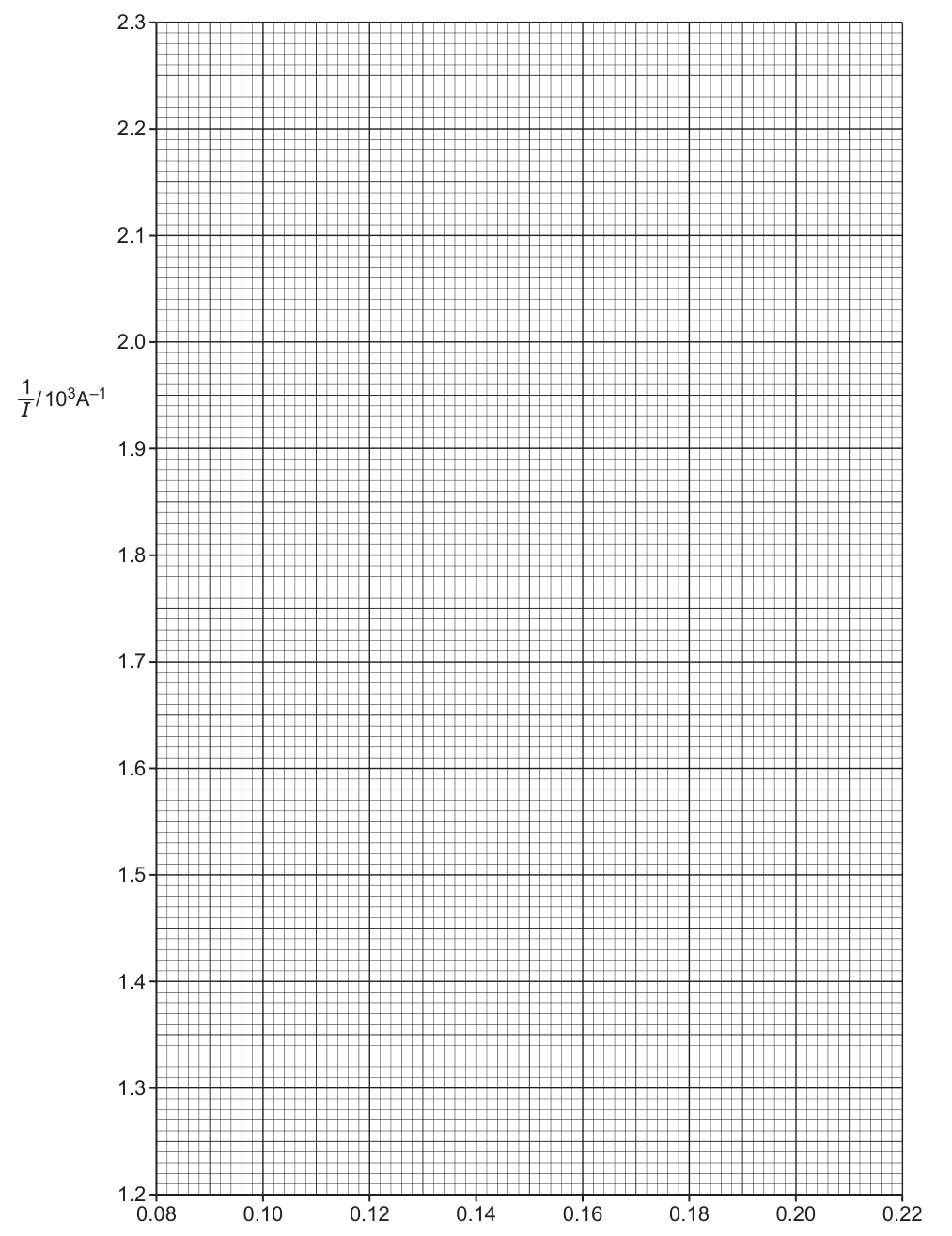
Points plotted (, ) with vertical error bars :
Graph plotted with the six points and vertical error bars using the calculated ± uncertainties in 1/I.
Background Concept
When plotting experimental data, you should:
- label axes with the quantity and unit,
- use a sensible scale that uses a large fraction of the grid,
- plot points as small crosses/dots,
- include error bars when uncertainties are given.
An error bar shows the range of possible true values based on the uncertainty. Here the uncertainty is in , so the error bars are vertical.
Understanding the Question
You must plot against using the values from your completed table, and include the error bars for from part (b).
Approach
- Put on the horizontal axis and on the vertical axis (as stated).
- Plot each coordinate pair from the table.
- For each point, draw a vertical error bar of length .
Step-by-Step Reasoning
Using the calculated values:
- At , plot and draw an error bar from to .
- Repeat similarly for the remaining five points.
Because is given to 3–4 s.f. and has no uncertainty stated, no horizontal error bars are required.
Key Takeaways
- Error bars go on the axis corresponding to the uncertain quantity.
- Always match the plotted quantities to the axis labels given in the question.
Common Mistakes
- Plotting instead of .
- Drawing horizontal error bars when only has an uncertainty.
- Forgetting the scale on the -axis and plotting values 1000 times too large.
Things to Be Careful About
- Make sure the points are plotted with consistent rounding (don’t over-round before plotting).
- Error bars should be centred on the plotted point and drawn neatly with small caps.
Draw the straight line of best fit and a worst acceptable straight line on your graph. Label both lines.
Answer
A straight line of best fit is drawn through the data.
A worst acceptable straight line is drawn such that it passes through all error bars.
Both lines are labelled.
Best-fit line and worst acceptable line drawn and labelled.
Background Concept
A best-fit line is the straight line that best represents the trend of the data (roughly equal scatter of points above and below). When uncertainties are shown with error bars, the “true” line could lie anywhere within those bars.
A worst acceptable line is an extreme line (steepest or shallowest) that is still consistent with the data within their error bars. This is used to estimate the uncertainty in the gradient and intercept.
Understanding the Question
You have already plotted points with vertical error bars. Now you must:
- draw the best-fit straight line,
- draw one worst acceptable straight line,
- label both on the graph.
Approach
- Draw the best-fit line: do not join point-to-point; draw one straight line.
- Draw a worst acceptable line: choose an extreme slope but ensure the line still passes through every vertical error bar (or at least is consistent with them as required by the paper).
- Label each line clearly (e.g. “best fit” and “worst”).
Step-by-Step Reasoning
- Best fit: aim for a balanced distribution of points above and below the line, and do not force it through the origin unless the data demand it.
- Worst acceptable: try drawing the steepest possible line (high on the left, low on the right) that still intersects each error bar; if that is not the greatest deviation from the best-fit gradient, try the shallowest possible line instead.
Key Takeaways
- Best-fit line uses the central trend.
- Worst acceptable line uses the uncertainty limits to estimate how much the gradient/intercept could vary.
Common Mistakes
- Drawing a “worst line” that ignores some error bars.
- Drawing two worst lines when only one is asked for.
- Not labelling the two lines (costs marks).
Things to Be Careful About
- Use a ruler; the lines must be straight.
- The worst acceptable line should be noticeably different in slope from the best-fit line, but still acceptable given the error bars.
Determine the gradient of the line of best fit. Include the absolute uncertainty in your answer.
gradient = ______
Working
Using two well-separated points on the best-fit line, e.g.
and :
Worst acceptable line (extreme):
Answer
(in units of )
8.15 ± 0.31 (in units of 10^3 A^-1)
Background Concept
The gradient of a straight-line graph is
To reduce the percentage reading error, you choose two points far apart on the drawn line (large triangle). When using a worst acceptable line, you do the same and then compare gradients.
The absolute uncertainty in the gradient (Paper 5 method) is typically taken as
where is the gradient of the worst acceptable line.
Understanding the Question
You must find:
- the gradient of the best-fit straight line on the graph of against ,
- and its absolute uncertainty using the worst acceptable line.
Approach
- Pick two widely separated points that lie on the best-fit line (not necessarily data points).
- Compute .
- Do the same for the worst acceptable line to get .
- Take .
Step-by-Step Reasoning
From the best-fit line, taking approximately and :
So
For a steepest acceptable line, you would use the extreme ends of the error bars to maximise slope (high at high , low at low ), giving a gradient around . Then
So the gradient is (in the plotted units).
Key Takeaways
- Use a large triangle on the line for gradient.
- Uncertainty comes from comparing best and worst acceptable lines.
Common Mistakes
- Using two adjacent points, giving a large reading uncertainty.
- Using by accident.
- Finding the gradient from the raw data points rather than from the drawn line.
Things to Be Careful About
- Make sure you are reading coordinates from the line itself.
- Keep consistent units: here the plotted values are already in .
Determine the -intercept of the line of best fit. Include the absolute uncertainty in your answer.
-intercept = ______
Working
For best-fit line, using with and a point on the line, e.g. :
Worst acceptable line gives intercept .
Answer
(in units of )
0.56 ± 0.04 (in units of 10^3 A^-1)
Background Concept
For a straight line
the -intercept is the value of when . On a graph you can often read it directly by extending the line to the -axis, or calculate it using a point on the line:
Uncertainty in intercept is found similarly to gradient, by comparing the best-fit and worst acceptable lines:
Understanding the Question
You need the intercept of the best-fit line for the plot of against , and the absolute uncertainty using the worst acceptable line.
Approach
- Find either by reading off at or by using .
- Find from the worst acceptable line in the same way.
- Take .
Step-by-Step Reasoning
Using and a point on the best-fit line such as :
For the worst acceptable line, the intercept might be about (from the line you drew). Then
So quote in the plotted units.
Key Takeaways
- Intercept can be found by extending to or by .
- Uncertainty is from best vs worst acceptable line.
Common Mistakes
- Reading the intercept from the wrong axis or at the wrong value.
- Using a data point rather than a point on the drawn best-fit line.
- Forgetting that the axis is scaled ().
Things to Be Careful About
- Choose a point on the line with clearly readable coordinates.
- Keep enough significant figures so that subtracting from is not dominated by rounding.
The e.m.f. of the battery is determined twice during the experiment. The values obtained are and .
Using your answers to (a), (c)(iii) and (c)(iv), determine the values of and . Include appropriate units.
= ______
= ______
Working
Mean e.m.f.:
From (a):
But graph uses , so
Hence
Answer
R = 4.7×10^4 Ω, Z = 3.2×10^3 Ω
Background Concept
From the linearised form
we can identify:
- gradient (of a graph of against ) is ,
- intercept is .
If the graph’s -axis is scaled (here it plots ), then the numerical gradient and intercept you read must be converted back to the unscaled values by multiplying by .
Understanding the Question
You have measured twice (5.6 V and 6.0 V), and from the graph you have the gradient and intercept (with the scaling). You must use these to calculate the actual resistor values and .
Approach
- Use the mean of the two readings as the best estimate.
- Convert the gradient and intercept from plotted units back to actual units by multiplying by .
- Use and .
Step-by-Step Reasoning
Mean e.m.f.:
Suppose the best-fit line has gradient and intercept on the axis labelled . This means
- actual gradient for is ,
- actual intercept is .
Now apply the identifications:
Similarly,
Key Takeaways
- Convert graph readings back to true units if the axis uses a scale factor.
- Gradient gives and intercept gives .
- Multiplying by returns resistances in ohms.
Common Mistakes
- Forgetting the factor from the -axis and obtaining resistances 1000 times too small.
- Using only one of the readings without any justification.
- Swapping and (mixing up gradient and intercept).
Things to Be Careful About
- Use consistent significant figures (typically 2–3 s.f.).
- Ensure you treat in volts and in so that and come out in .
Determine the percentage uncertainty in your value of .
percentage uncertainty = ______
Working
For and :
From (c)(iii):
Since ,
Answer
7.2%
Background Concept
If a quantity is found by multiplying two measured quantities, e.g.
then the percentage (fractional) uncertainties add:
To estimate uncertainty in a mean from two repeated readings, a common Paper 5 method is to take half the range:
Understanding the Question
You found from the gradient and . The gradient has an uncertainty from the best/worst line method, and was measured twice (5.6 V and 6.0 V). You must find the percentage uncertainty in .
Approach
- Use the mean as the best estimate and half the range as .
- Convert both and into percentage uncertainties.
- Add them because is proportional to the product .
Step-by-Step Reasoning
Mean e.m.f.:
Uncertainty in (half-range):
Percentage uncertainty in :
From the graph, suppose
Then
Since (after handling the axis scaling consistently),
Key Takeaways
- For products, percentage uncertainties add.
- Two repeated readings can give an uncertainty estimate using half the range.
- Use the uncertainty in the gradient from best vs worst lines.
Common Mistakes
- Using the full range instead of half-range .
- Combining absolute uncertainties directly (must use percentage for multiplication).
- Ignoring the uncertainty in even though repeat values are given.
Things to Be Careful About
- Quote the final percentage uncertainty to a sensible number of significant figures (usually 2 s.f.).
- Make sure you use the same best estimate of in the uncertainty calculation as you used when calculating .
The experiment is repeated with 20 resistors, each of resistance , connected in parallel between P and Q. Determine the total current in the circuit.
= ______
Working
Using , , and :
Answer
1.04×10^-3 A
Background Concept
The total resistance in series adds. Here, the circuit has:
- a parallel network of identical resistors of resistance , giving equivalent resistance ,
- in series with a fixed resistor .
So the total resistance is
and with negligible internal resistance the current is
Understanding the Question
You increase the number of parallel resistors to (keeping the same for each resistor). Using your previously determined values of and and the battery e.m.f. , you must predict the new total current .
Approach
- Calculate the equivalent parallel resistance for .
- Add to get the total series resistance.
- Use .
Step-by-Step Reasoning
With :
Total resistance:
Current:
Key Takeaways
- More parallel resistors reduces , increasing current.
- Use series-plus-parallel simplification before substituting into .
Common Mistakes
- Using instead of for parallel resistors.
- Forgetting that is in series and must be added to .
- Mixing and units.
Things to Be Careful About
- Keep values in when adding resistances.
- Quote in amperes; check order of magnitude (here about matches the earlier – scale).