Physics 9702/52 — February/March 2025
Cambridge A-Level · Planning, Analysis and Evaluation · worked solutions for every part, with the mark scheme
Topics Analysis, Conclusions and Evaluation · Planning
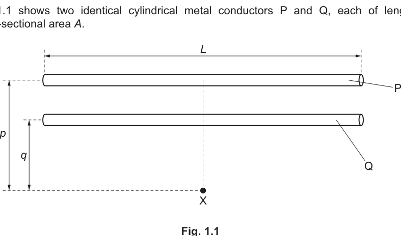
Fig. 1.1 shows two identical cylindrical metal conductors P and Q, each of length and cross-sectional area .
The conductors are placed parallel to each other. The perpendicular distance from the midpoint of P to point X is . The perpendicular distance from the midpoint of Q to point X is .
The two conductors are electrically connected in parallel. This parallel combination is connected in series to a power supply and a resistor. The potential difference between the ends of P is the same as the potential difference between the ends of Q.
The magnetic flux density at X due to the currents in the conductors is .
It is suggested that is related to by the relationship
where and are constants.
Plan a laboratory experiment to test the relationship between and .
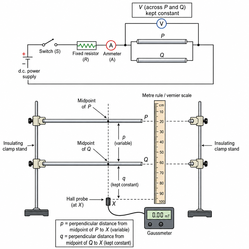
Draw a diagram showing the arrangement of your equipment.
Explain how the results could be used to determine values for and .
In your plan you should include:
- the procedure to be followed
- the measurements to be taken
- the control of variables
- the analysis of the data
- any safety precautions to be taken.
Variables
- Independent variable: (perpendicular distance from midpoint of conductor P to point X).
- Dependent variable: magnetic flux density at X.
- Control variables: (keep fixed), across P and Q (keep constant), same conductors so and constant, point X on the perpendicular line through the midpoints, orientation of Hall probe, ambient magnetic field.
Apparatus
Two identical straight cylindrical conductors P and Q on insulating clamps, low-voltage d.c. power supply, series resistor, switch, ammeter, voltmeter across the parallel combination, Hall probe / gaussmeter, metre rule / vernier scale to measure and , micrometer screw gauge for diameter (to find ).
Procedure and measurements
- Mount Q fixed. Mark the midpoint of Q and place the Hall probe at point X a fixed perpendicular distance from this midpoint (measure with a rule and keep the probe position fixed).
- Mount P parallel to Q with its midpoint on the same perpendicular line through X. Adjust the separation so that the perpendicular distance from P’s midpoint to X is .
- Connect P and Q in parallel. Connect this parallel pair in series with the resistor, ammeter and power supply.
- Set the supply so that the potential difference across P (and Q) is a chosen constant value (monitor with the voltmeter). Keep the same for all readings.
- For each value of :
- measure and record (and check unchanged),
- measure with current flowing,
- measure background field with switch open,
- take .
- Take at least 6 values of over a wide range, repeating readings and averaging.
- Measure of a conductor and diameter to obtain .
Analysis of data (to find and )
With constant, the suggested relationship
So plot a graph of (y-axis) against (x-axis).
- Gradient
- Intercept
Hence
and
Use a best-fit line and worst acceptable line to estimate uncertainties in and , and propagate to uncertainties in and .
Safety
- Use low voltage and a series resistor to limit current.
- Conductors may heat up: switch off between readings / keep current small and avoid touching metal.
- Keep leads insulated and secure to prevent short circuits.
See working
Background Concept
A current in a long straight conductor produces a magnetic field (and hence magnetic flux density ) around it. In many experiments, we do not calculate from first principles; instead we measure with a Hall probe and test whether a suggested mathematical relationship matches the data.
Here the suggested model is
where:
- is the magnetic flux density at point X,
- and are perpendicular distances from the midpoints of P and Q to X,
- is the p.d. across each conductor (same because P and Q are in parallel),
- and are the cross-sectional area and length of each conductor,
- and are constants to be found experimentally.
A key skill in Paper 5 planning is to (i) decide what to vary and what to keep constant, (ii) decide what to measure and how, and (iii) choose a graph that gives a straight line so constants can be extracted from a gradient and intercept.
Understanding the Question
You must plan an experiment to test how depends on for two identical parallel conductors connected in parallel, and then explain how your results can be used to determine and .
Important details from the stem:
- P and Q are identical (same and ), and each has p.d. across it.
- at X is due to the currents in both conductors.
- The proposed equation contains both and , so if you vary you should ideally keep constant; otherwise the second term changes too and the test becomes ambiguous.
Approach
- Make the independent variable and measure at X for many values of .
- Keep constant by fixing the position of X relative to conductor Q (e.g. keep Q and the Hall probe fixed) and moving conductor P to change .
- Keep constant and monitor it with a voltmeter across the parallel pair.
- Remove systematic effects:
- subtract the background magnetic field (Earth field and nearby equipment) by measuring with current off.
- keep the Hall probe orientation fixed.
- Linearise: with constant, should be linear in . A straight-line graph allows and to be extracted from gradient and intercept.
Step-by-Step Reasoning
1) Set up a workable geometry
You need P and Q straight, parallel, and with their midpoints aligned so that and are genuinely the perpendicular distances from the midpoints to point X.
A practical way:
- Clamp Q fixed on insulating supports.
- Place the Hall probe at X a fixed distance below Q (or to the side—any perpendicular direction is fine as long as you measure it consistently). Measure this distance once as .
- Clamp P parallel to Q, and adjust its position so its midpoint lies on the same perpendicular line to X. Then changing the separation between P and Q changes while leaving unchanged.
2) Circuit arrangement and keeping constant
Because P and Q are in parallel, they share the same p.d. . Put the parallel combination in series with:
- a resistor (current limiting),
- an ammeter (optional but useful for checking current is not drifting),
- a switch,
- the d.c. supply.
Place a voltmeter across the parallel combination so you can set and maintain a constant for all readings.
3) Measurements to take
For each :
- Measure with a ruler/vernier (record uncertainty).
- Measure with the Hall probe when current flows.
- Measure with the switch open to get the background field.
- Calculate .
Also measure the constants needed for later:
- (length of each conductor) with a rule.
- Diameter with a micrometer; then compute
Take multiple readings of for each and average, because can fluctuate due to probe noise and small movements.
4) Control of variables
To make it a fair test of “ vs ”:
- Keep fixed (do not move Q or X).
- Keep constant (adjust the supply if needed and record each time).
- Keep the Hall probe at the same orientation (Hall probes measure the component of along a specific axis).
- Keep conductors straight and parallel; keep midpoints aligned with X.
- Reduce heating (temperature rise changes resistance and could change currents even if supply settings drift). Use low current and switch off between readings.
5) Linearising and extracting and
Start from the given model:
If , , , are constants during the experiment, rewrite as
This is in the straight-line form with:
- gradient
- intercept
So:
and, using to eliminate ,
A straight line within uncertainty supports the suggested relationship.
6) Uncertainties (what you would write in Paper 5)
- Add error bars in (from probe resolution and repeat scatter) and in (from uncertainty in ).
- Find uncertainty in gradient and intercept using a worst acceptable line.
- Then propagate:
- fractional uncertainty in is the sum of fractional uncertainties in , , , as appropriate (often is from so ).
- fractional uncertainty in comes mainly from uncertainties in , , and .
Key Takeaways
- In planning, make one variable change (here ) while keeping all others in the equation constant (especially ).
- Use background subtraction () to reduce systematic error.
- Turn a proposed relationship into a straight-line graph; use gradient and intercept to determine constants ( and ).
- For Paper 5, you must describe measurements, controls, analysis, and safety clearly and specifically.
Common Mistakes
- Varying by moving point X, causing to change as well (then you are not testing the stated dependence cleanly).
- Forgetting that a Hall probe measures one component of and rotating it between readings.
- Not measuring/subtracting the background magnetic field.
- Plotting against instead of against (loses the linear method for finding constants).
- Giving a graph method but not stating explicitly how and are calculated from gradient/intercept.
Things to Be Careful About
- Keep the conductors and the probe away from magnetic materials and other current-carrying wires (stray fields).
- Ensure the “midpoint” distances and are measured from the correct locations (mark midpoints).
- Avoid very small where the Hall probe might be too close to the conductor (risk of contact, poor geometry, very large gradients in ).
- Use consistent SI units (convert cm to m before calculating if needed).
- Heating: if temperature rises, resistance changes and currents may drift; keep current low and take readings quickly.
A student investigates the cooling of a liquid in a beaker.
The temperature of the laboratory is measured using a thermometer.
Hot water is added to an insulated beaker, as shown in Fig. 2.1.
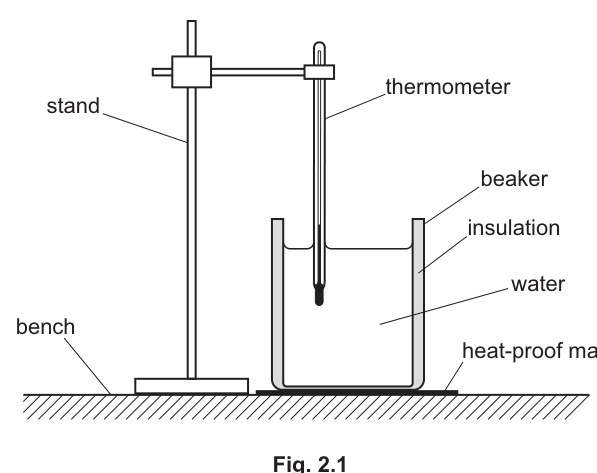
The thermometer measures the temperature of the water. At time the temperature of the water is .
A series of readings of and are taken.
It is suggested that and are related by the equation
where is the temperature at and is a constant.
A graph is plotted of on the -axis against on the -axis.
Determine expressions for the gradient and -intercept.
gradient = ______
-intercept = ______
Working
Given
Take ln:
Comparing with for a graph of against :
Answer
gradient
-intercept
gradient = -1/K; y-intercept = ln(θ0 − θR)
Background Concept
Cooling that follows Newton’s law of cooling can produce an exponential approach to room temperature. An exponential form like
is hard to analyse directly on a straight-line graph. A standard technique is to linearise by taking natural logs so that we can use
where the gradient and intercept can be read from a straight line.
Understanding the Question
You are told to plot a graph of (vertical axis) against (horizontal axis). The question asks: once you have rewritten the given cooling equation into the form , what are the expressions for:
- the gradient
- the intercept .
Approach
- Subtract from both sides so the exponential is by itself.
- Take of both sides.
- Rearrange so it looks like .
- Read off gradient and intercept.
Step-by-Step Reasoning
Start with:
Subtract :
Now take natural logs:
and since :
Compare with where and :
- .
Key Takeaways
- Exponentials are linearised by taking logs.
- After linearisation, gradient and intercept come from direct comparison with .
Common Mistakes
- Forgetting to subtract before taking .
- Writing gradient as or without showing it is specifically .
- Giving intercept as instead of .
Things to Be Careful About
- The log is of , not of .
- When plotting , the division by is just to make the argument dimensionless; the algebraic intercept still corresponds to (numerically the same as if you treat the temperature difference in °C as a pure number).
Values of and are given in Table 2.1.
Table 2.1
| / min | / °C | / °C | |
|---|---|---|---|
| 6.0 | 75.0 0.5 | ||
| 12.0 | 64.5 0.5 | ||
| 18.0 | 57.0 0.5 | ||
| 24.0 | 50.0 0.5 | ||
| 30.0 | 44.5 0.5 | ||
| 36.0 | 41.0 0.5 |
The value of is .
Calculate and record values of and in Table 2.1. Include the absolute uncertainties in and .
Working
For :
Absolute uncertainty:
For with :
Completed values (to suitable d.p.):
| / min | / °C | abs unc in | |
|---|---|---|---|
Answer
Values recorded in Table 2.1 as above.
See working
Background Concept
When you calculate a new quantity from measurements, you must also estimate its uncertainty.
Two key rules used here:
-
Addition/subtraction: absolute uncertainties add.
If , then typically
- Natural log: for , a small change satisfies
This comes from differentiation: .
Understanding the Question
You are given and (each has ) and . You must fill two extra columns:
- and its absolute uncertainty
- and its absolute uncertainty (for plotting error bars later).
Approach
For each row:
- Compute .
- Uncertainty in is .
- Compute (numerically this is just if is in °C).
- Compute .
Step-by-Step Reasoning
Example for :
- Difference:
- Absolute uncertainty in difference:
- Log value:
- Uncertainty in log:
Repeat the same process for each row; the uncertainty in grows as the water cools because gets smaller, so increases.
Key Takeaways
- Subtraction: add absolute uncertainties.
- For , the absolute uncertainty is approximately the fractional uncertainty in .
- Error bars should reflect these calculated values.
Common Mistakes
- Using instead of .
- Calculating instead of .
- Giving uncertainty in as (log uncertainties are unitless and usually much smaller).
Things to Be Careful About
- Keep consistent decimal places for (here to is appropriate because inputs are to ).
- values should be to at least 3 decimal places so plotting is accurate.
- The argument of a logarithm should be dimensionless; writing makes this explicit.
Answer
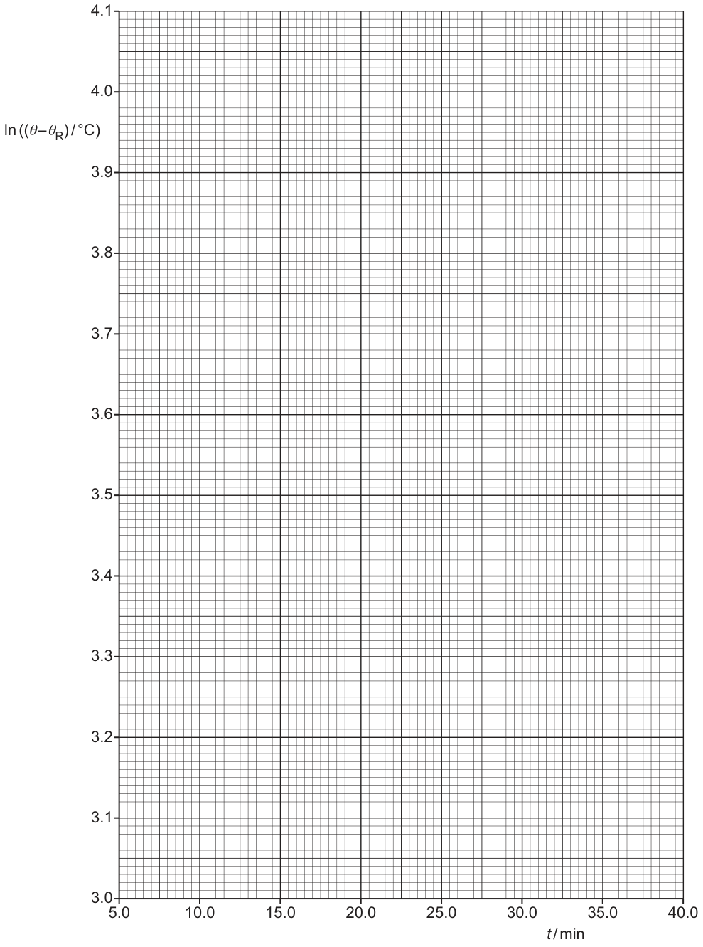
Points plotted on Graph 2.1 at:
Vertical error bars drawn for of:
respectively.
Graph plotted with y-error bars
Background Concept
A straight-line graph is used to test whether a linear relationship holds and to extract constants. When there are measurement uncertainties, points should be plotted with error bars so you can judge how well a straight line fits within uncertainty.
Understanding the Question
You must use your calculated values and their absolute uncertainties from (b), then:
- plot against on the provided grid
- include vertical error bars of size for each point.
Approach
- Put each point at its coordinate.
- For each, draw a vertical line from to (horizontal “caps” are optional unless specifically required).
- Ensure the plotted points are small, neat crosses or dots so the best-fit line can be judged.
Step-by-Step Reasoning
Using the completed table:
- At , plot .
- Draw an error bar from to .
Repeat for all six points. Because the values increase as temperature difference decreases, the later points (larger ) should have visibly larger error bars.
Key Takeaways
- Plot the transformed variable actually requested ().
- Error bars are based on the uncertainty in the transformed variable, not the original temperature directly.
Common Mistakes
- Plotting against instead of against .
- Using the same-sized error bar for every point (here they are different).
- Plotting using too few decimal places so points are shifted noticeably.
Things to Be Careful About
- Axes: on and on .
- Error bars must be centred on the plotted point.
- Do not join the points dot-to-dot; a best-fit line is drawn in (c)(ii).
Draw the straight line of best fit and a worst acceptable straight line on your graph. Label both lines.
Answer
A straight line of best fit drawn through the plotted points.
A worst acceptable straight line drawn (steepest/shallowest that still passes through all error bars) and both lines labelled clearly.
Best-fit line and worst acceptable line drawn and labelled
Background Concept
When data should be linear, experimental scatter means points will not lie exactly on a straight line. The line of best fit represents the most reasonable overall trend.
To estimate uncertainty in gradient/intercept from a graph, Paper 5 often uses a worst acceptable line: the steepest (or shallowest) straight line that is still consistent with the plotted points within their error bars.
Understanding the Question
After plotting points and vertical error bars, you must draw:
- one best-fit straight line
- one worst acceptable straight line
and label them.
Approach
- Best-fit line: balance the points above and below; do not force it through every point.
- Worst acceptable line: pivot to make the line as different as possible (steepest or shallowest) while still intersecting every error bar.
- Label each line so it is clear which is which.
Step-by-Step Reasoning
- Draw the best-fit line first: it should run through the middle of the scatter and follow the overall downward trend.
- Then draw the worst acceptable line:
- Choose whether you will draw the shallowest or steepest line relative to the best fit (either is acceptable; you normally pick whichever gives the larger change in gradient).
- Make sure your line still passes through (or at least touches) every vertical error bar.
This second line is not “another best fit”; its purpose is to create a plausible extreme so that the difference from the best-fit gradient/intercept can be used as an uncertainty.
Key Takeaways
- Worst acceptable line must be consistent with all error bars.
- Labelling is essential so the examiner can see which line you used for uncertainties.
Common Mistakes
- Drawing a curve instead of a straight line.
- Drawing a worst line that misses one or more error bars.
- Forgetting to label the lines.
Things to Be Careful About
- Use a ruler.
- Extend lines sufficiently so you can read intercept at and choose widely separated points for gradient in (c)(iii)/(c)(iv).
Determine the gradient of the line of best fit. Include the absolute uncertainty in your answer.
gradient = ______
Working
Using two widely spaced points on the best-fit line (e.g. at and ):
Worst acceptable gradient (from worst acceptable line) e.g.
Absolute uncertainty:
Answer
(-3.10 ± 0.24) × 10^-2 min^-1
Background Concept
For a straight-line graph, the gradient is
Using points far apart reduces percentage reading error.
To estimate uncertainty graphically:
- find from the best-fit line
- find from the worst acceptable line
- take an absolute difference as the uncertainty (some schemes use half-range if you draw both steepest and shallowest; if only one worst line is drawn, use the difference from best).
Understanding the Question
You must read the gradient of your best-fit line from the graph of against , and include an absolute uncertainty using your worst acceptable line.
Approach
- Pick two points on the best-fit line (not necessarily plotted data points) that are widely separated.
- Calculate .
- Repeat using the worst acceptable line to get .
- Uncertainty is the difference between them.
Step-by-Step Reasoning
Suppose from the best-fit line you can read two convenient points around and . Compute
The gradient should be negative because decreases with time.
Then read two points from the worst acceptable line in the same way to obtain . The uncertainty is
and quote the gradient as with unit .
Key Takeaways
- Use large triangles / widely spaced points for gradients.
- Uncertainty comes from the range of acceptable lines given the error bars.
Common Mistakes
- Using (inverted gradient).
- Choosing two points very close together.
- Forgetting the gradient is negative.
- Quoting no unit; here it must be .
Things to Be Careful About
- Use points on the drawn line, not the raw data points unless they lie on the line.
- Keep consistent significant figures: uncertainty typically to 1–2 s.f., gradient to match.
Determine the -intercept of the line of best fit. Include the absolute uncertainty in your answer.
-intercept = ______
Working
From best-fit line, extrapolate to :
From worst acceptable line, intercept e.g.
Absolute uncertainty:
Answer
4.21 ± 0.04
Background Concept
For a straight line , the -intercept is the value of when . On a graph, you find it by extending the line to cross the -axis (or by calculating from a point on the line).
Uncertainty in the intercept can be estimated by comparing the intercepts from the best-fit and worst acceptable lines.
Understanding the Question
You need the intercept of your best-fit line on the graph of vs , and you must include an absolute uncertainty.
Approach
- Extend the best-fit line back to and read off .
- Extend the worst acceptable line back to and read off .
- Take .
Step-by-Step Reasoning
- The intercept is often outside the plotted range of values, so you may need to extrapolate.
- Use a ruler and extend carefully; small angle changes can cause noticeable changes in .
- Once you have both intercepts, the difference is your absolute uncertainty.
Key Takeaways
- Intercept is a read-off at .
- Worst acceptable line provides the uncertainty estimate.
Common Mistakes
- Reading the intercept at the left edge of the graph instead of at .
- Forgetting to include uncertainty.
- Mixing up intercept with the value at .
Things to Be Careful About
- Quote to match the precision justified by the graph scale (typically 2 d.p. at most here).
- Ensure you use the same origin as the axis label (minutes).
Using your answers to (a), (c)(iii) and (c)(iv), determine the values of and . Include appropriate units.
= ______
= ______
Working
From (a): gradient and intercept .
With :
With :
Answer
K = 32.3 min; θ0 = 85.6 °C
Background Concept
After linearising an exponential relationship, the straight-line graph constants map back to the physical constants.
Here:
So on a plot of vs :
- gradient
- intercept .
Understanding the Question
You have already found (from your graph):
- gradient with unit
- intercept (dimensionless)
Using these and the expressions from (a), you must calculate numerical values for:
- (in minutes)
- (in °C).
Approach
- Rearrange to get .
- Rearrange by exponentiating: .
- Add to obtain .
Step-by-Step Reasoning
- Since is negative, will come out positive because of the minus sign:
- For the intercept:
This gives the initial temperature difference above room temperature. Finally:
Key Takeaways
- Gradient gives the time constant: .
- Intercept gives the initial excess temperature: .
Common Mistakes
- Using instead of .
- Forgetting to exponentiate the intercept.
- Forgetting to add to get .
Things to Be Careful About
- Units: must be in minutes because was in minutes.
- Make sure the calculator is in natural log/exponential mode (use , not ).
Working
From .
With :
Combine with :
Answer
absolute uncertainty
3.2 °C
Background Concept
Uncertainty propagation depends on the mathematical operation.
- For a sum , a common Paper 5 method is to add absolute uncertainties:
- For an exponential , use the small-change approximation from differentiation:
so
Understanding the Question
You found in (d)(i), and now you must find the absolute uncertainty in .
Since
the uncertainty comes from both and the intercept .
Approach
- Convert intercept uncertainty into uncertainty in using .
- Add the room-temperature uncertainty to get .
Step-by-Step Reasoning
- First compute (this is ).
- Then compute
because a small change in changes proportionally.
- Finally, because is a sum,
This gives an absolute uncertainty in °C.
Key Takeaways
- Exponential uncertainty: .
- Sum uncertainty: add absolute uncertainties.
Common Mistakes
- Treating as equal to (wrong units and wrong magnitude).
- Forgetting that has its own uncertainty.
- Quoting the uncertainty to too many significant figures.
Things to Be Careful About
- is dimensionless, but must be in °C.
- If your uncertainty is found using a different worst acceptable line, your numerical uncertainty will differ; method marks come from using the correct propagation.
Working
For ,
Using with and :
Answer
75.5 min
Background Concept
Once you have a model (from your straight-line fit), you can predict values by substitution.
From the linearised equation:
you can find the time for any temperature by:
- computing for that temperature
- rearranging for :
Alternatively, you can rearrange the original exponential directly with logs; both approaches are equivalent.
Understanding the Question
You are asked for the time when the water reaches , using the relationship you have established (i.e. using your determined constants from the graph).
Approach
- Compute the temperature difference above room: .
- Take the natural log to find the corresponding value on the graph.
- Use the straight-line equation with your best-fit gradient and intercept to solve for .
Step-by-Step Reasoning
- At , the excess above room is .
- The plotted variable is
- Substitute into and rearrange:
Because is negative and , the time comes out positive, as expected.
Key Takeaways
- You can use the linear graph form to predict times/temperatures quickly.
- Always use , not .
Common Mistakes
- Using instead of .
- Sign error when dividing by a negative gradient.
- Using base-10 logarithms instead of natural logs.
Things to Be Careful About
- Ensure consistent units: in minutes because the gradient is in .
- If you use rounded values of and , your may differ slightly; the key is correct method and sensible rounding.