Physics 9702/53 — October/November 2024
Cambridge A-Level · Planning, Analysis and Evaluation · worked solutions for every part, with the mark scheme
Topics Analysis, Conclusions and Evaluation · Planning
A thin cylindrical bar magnet of length and cross-sectional area is attached to a block.
An identical magnet is attached to a trolley, as shown in Fig. 1.1.
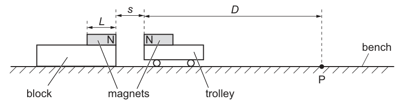
The trolley is held so that the separation of the N poles of the two magnets is .
Point P is a distance from the N pole of the magnet on the stationary trolley.
The trolley is released. The speed of the trolley at point P is determined using one light gate.
It is suggested that is related to by the relationship
where is the magnetic flux density at the N pole of one of the magnets, is the mass of the trolley, and and are constants.
Plan a laboratory experiment to test the relationship between and .
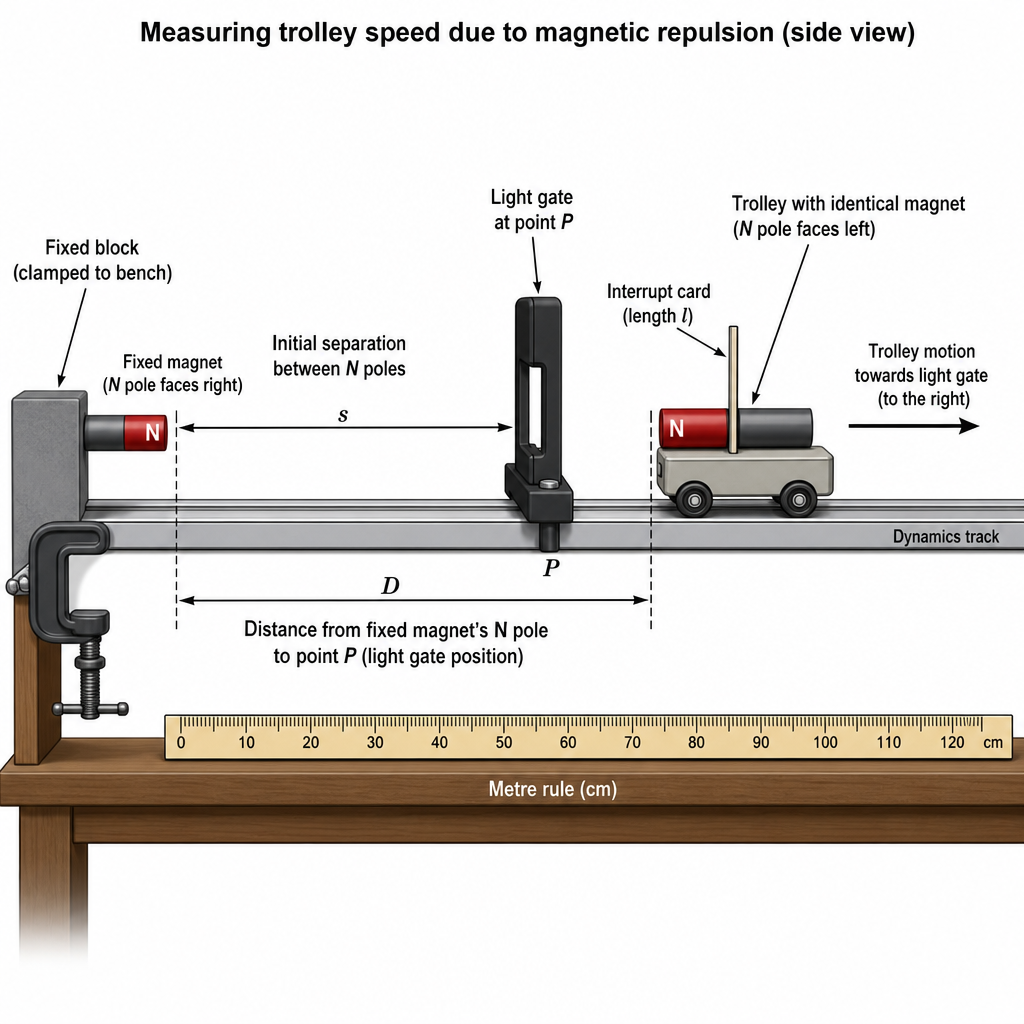
Draw a diagram showing the arrangement of your equipment.
Explain how the results could be used to determine values for and .
In your plan you should include:
● the procedure to be followed
● the measurements to be taken
● the control of variables
● the analysis of the data
● any safety precautions to be taken.
Answer
Variables
- Independent variable: separation of N poles, .
- Dependent variable: trolley speed at point , .
- Control variables: (position of /light gate), same two identical magnets (so , , constant), track angle/level (to keep gravitational component constant), starting from rest with no push, trolley mass constant.
Apparatus
- Low-friction dynamics track and trolley.
- Two identical thin cylindrical bar magnets, one fixed to a block/clamp, one fixed to trolley (N poles facing).
- Light gate + data logger/timer, interrupt card of known length on trolley.
- Metre rule / vernier calipers (for , , magnet dimensions), top-pan balance (for ).
- (Optional if required) Hall probe/gaussmeter to measure at the pole.
Procedure and measurements
- Level the track (so trolley does not drift when magnets are far apart).
- Fix the block with magnet at one end. Mark point on the track a distance from the N pole of the fixed magnet and clamp the light gate at .
- Measure and record .
- Attach an interrupt card of length to the trolley; connect light gate to timer to measure the time for the card to pass.
- Set an initial separation between the two N poles (measure with a rule/callipers along the track axis). Hold the trolley at this position using a card/spacer and release without a push.
- Record at the light gate and calculate .
- Repeat at least 3 times for the same and take mean .
- Repeat for at least 6 different values of over a suitable range (ensuring no collision).
- Measure of the trolley + attached magnet. Measure magnet length and diameter to obtain cross-sectional area . Measure with a Hall probe at a fixed position at the pole (same for both magnets).
Analysis (test the relationship and find and )
Rearrange:
Let
Then
- For each run, calculate and .
- Plot a graph of (vertical) against (horizontal).
- A straight line supports the relationship.
- Gradient so
- Intercept so
(Use a best-fit line; estimate uncertainties in and using a worst acceptable line if required.)
Safety
- Strong magnets: keep fingers clear to avoid trapping; keep away from phones/cards/pacemakers.
- Prevent trolley/magnets colliding by using a stop/catcher; keep face/hands clear of moving trolley.
See working
Background Concept
The suggested relationship is
Here is the speed of the trolley when it reaches a fixed point a distance from the fixed magnet’s N pole. The right-hand side depends on the initial separation between the two N poles when the trolley is released.
To test a relationship experimentally, we typically:
- Vary one quantity (independent variable) over a good range.
- Measure the response (dependent variable) reliably, with repeats.
- Keep other quantities constant (controls), so any change in the dependent variable can be attributed to the independent variable.
- Convert the equation into a straight-line form so we can use a graph to check linearity and determine constants from the gradient/intercept.
A light gate gives speed at a point by measuring how long an interrupt card blocks the beam. If the card length is and the blocking time is , then
Understanding the Question
You are asked to plan an experiment where:
- you set different initial separations between the magnets,
- release the trolley, and
- measure its speed when it passes a fixed point .
You must also explain how to process your data to determine numerical values for the constants and .
Crucially, the relationship contains , so plotting directly against will not give a straight line. The clue is to use the given equation and rearrange it for a linear graph.
Approach
- Choose variables: make the independent variable; measure at point as the dependent variable.
- Fix the geometry: keep point the same for every run, so is constant. Clamp the light gate at .
- Make other terms constant: use the same trolley and the same pair of identical magnets, with fixed orientation, so , and do not change. Keep the track level so the energy change is due to magnet interaction rather than gravity.
- Collect data carefully: measure using a light gate with an interrupt card; repeat each value and average.
- Linearise: define
so a plot of vs should be a straight line.
6. Extract constants: gradient gives (after dividing by ), and intercept gives .
Step-by-Step Reasoning
-
Set up a low-friction track and level it. If the track is not level, the trolley gains/loses gravitational potential energy, changing in a way unrelated to .
-
Fix one magnet to a block/clamp so it cannot move. Attach the second identical magnet to the trolley so the N poles face each other (as in the question).
-
Fix point by measuring a distance from the fixed magnet’s N pole along the track and clamping the light gate at this location. Then is controlled for every run.
-
Measure speed at :
- attach an interrupt card of known length to the trolley,
- the light gate measures the time the beam is blocked,
- calculate .
Repeating each run reduces random timing variation.
-
Vary :
- use a ruler/vernier calipers to set and measure the initial separation between the two N poles along the line of motion,
- release the trolley from rest without pushing (a thin card spacer can help you hold and release consistently).
-
Repeat for a range of values (e.g. 6–10 values). A wider range helps reveal whether the proposed dependence is correct.
-
Measure constants needed to calculate :
- using a balance (trolley + attached magnet),
- and magnet diameter with vernier calipers so
- with a Hall probe/gaussmeter at a fixed, defined location at the pole (and keep that method identical for all measurements).
- Linearise and plot:
For each , compute
and from the mean speed,
Then plot against . If the suggested model is correct, the points should lie close to a straight line.
- Determine and :
From
- gradient , hence
- y-intercept , hence
- Uncertainty (good practice in Paper 5): estimate uncertainties in , , and ; propagate to and if required. For the graph, draw a best-fit line and a worst acceptable line to estimate uncertainties in gradient/intercept (and therefore in and ).
Key Takeaways
- Good plans clearly state independent/dependent/control variables and how controls are maintained.
- Light gates measure speed at a point via .
- Testing a relationship often means rearranging to and using a straight-line graph.
- Constants in a model commonly come from gradient and intercept; here comes from the gradient after dividing by known constants, and comes from the (negative) intercept.
Common Mistakes
- Plotting against directly (won’t be linear for an law).
- Forgetting to keep fixed (moving the light gate between runs changes ).
- Measuring from the wrong reference points (must be N-pole to N-pole along the axis).
- Releasing the trolley with a push (adds extra kinetic energy, increasing ).
- Not stating how and are obtained from the graph (must link gradient/intercept to the constants).
Things to Be Careful About
- Collision risk: for small the repulsion is strong; ensure the trolley does not crash into the block and that magnets cannot detach.
- Consistency of : near a magnet pole varies rapidly with position; define a fixed measurement position if measuring with a Hall probe.
- Units: use SI units (e.g. and in m, in kg, in m s) so the plotted quantities are consistent.
- Graph quality: use a wide scale, plot enough points, and use large triangles for gradients; if asked for uncertainty, use worst acceptable line methods.
A student investigates an electrical circuit. A power supply of electromotive force (e.m.f.) and negligible internal resistance is connected in series to three resistors, each of resistance .
A cell, an ammeter and a resistor of resistance are connected in parallel across one of these resistors, as shown in Fig. 2.1.
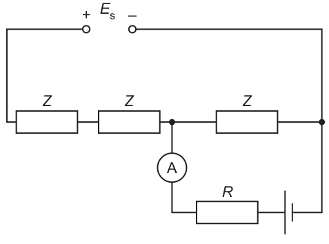
The current is measured by the ammeter for different values of .
It is suggested that and are related by the equation
where is the e.m.f. of the cell.
A graph is plotted of on the -axis against on the -axis.
Determine expressions for the gradient and -intercept.
gradient = ______
-intercept = ______
From
So
With -axis as (so ):
Answer
gradient
-intercept
gradient = 3000/(3E - Es), y-intercept = 2Z/(3E - Es)
Background Concept
To test a suggested relationship experimentally, we often rearrange it into the straight-line form
where is the gradient and is the -intercept. If a graph of against is a straight line, the relationship is supported, and values of physical constants can be found from and .
Here, the suggested equation is
where and are e.m.f.s, is current, and and are resistances.
Understanding the Question
You are told the student plots (vertical axis) against (horizontal axis). You must rearrange the given equation into an expression for in terms of , then identify:
- the coefficient of (this becomes the gradient),
- the constant term (this becomes the -intercept).
Also note the graph uses on the -axis, so the numerical gradient is different by a factor of compared with using in .
Approach
- Rearrange to make the subject.
- Compare with .
- Adjust if the plotted variable is in rather than .
Step-by-Step Reasoning
Starting with
divide both sides by :
Split the fraction:
So if the -axis were in , then
But the graph uses , so :
Hence
and the intercept is unchanged:
Key Takeaways
- Rearrange into to read off gradient and intercept.
- Always check what units/scaling are used on graph axes (here introduces a factor of ).
Common Mistakes
- Giving gradient as even though the -axis is in .
- Mixing up intercept and gradient terms.
Things to Be Careful About
- The intercept does not change when changing the unit of the -axis; only the gradient changes.
- Keep and in volts and resistances consistently when later using the gradient/intercept to find constants.
Values of and are given in Table 2.1.
Table 2.1
| 1.50 | ||
| 1.75 | ||
| 1.92 | ||
| 2.22 | ||
| 2.48 | ||
| 2.72 |
Calculate and record values of in Table 2.1.
Include the absolute uncertainties in .
For ,
(using in A and )
Values:
- : ,
- : ,
- : ,
- : ,
- : ,
- : ,
Answer
values and absolute uncertainties as above (to be entered in Table 2.1).
1/I = 5.15e3, 5.56e3, 5.81e3, 6.25e3, 6.67e3, 6.94e3 A^-1 with uncertainties ±5.3e1, ±6.2e1, ±6.8e1, ±7.8e1, ±8.9e1, ±9.6e1 A^-1
Background Concept
If a measured quantity has an absolute uncertainty , then for a derived quantity
the uncertainty can be found using differentiation (or the standard rule for powers):
This gives an absolute uncertainty in the same units as (here, ).
Understanding the Question
The table gives in with . You must:
- convert each into amperes,
- calculate in ,
- calculate the absolute uncertainty in using .
Approach
For each row:
- Use .
- Compute .
- Use and calculate .
Step-by-Step Reasoning
Example for :
Convert:
Reciprocal:
Uncertainty (with ):
Repeat the same steps for each current value. Notice that as gets smaller, gets larger and its uncertainty also gets larger (because ).
Key Takeaways
- Always convert to SI units before calculating.
- For reciprocals, absolute uncertainty is .
- Smaller currents lead to larger uncertainty in .
Common Mistakes
- Using (that is a fractional uncertainty idea, not correct for the absolute uncertainty here).
- Forgetting to convert to A, giving answers off by a factor of .
- Writing uncertainties as percentages when the question asks for absolute uncertainties.
Things to Be Careful About
- Quote in (not ).
- Keep rounding sensible: uncertainties to 1 or 2 significant figures, and the value of to a matching decimal place/significant figure.
Answer
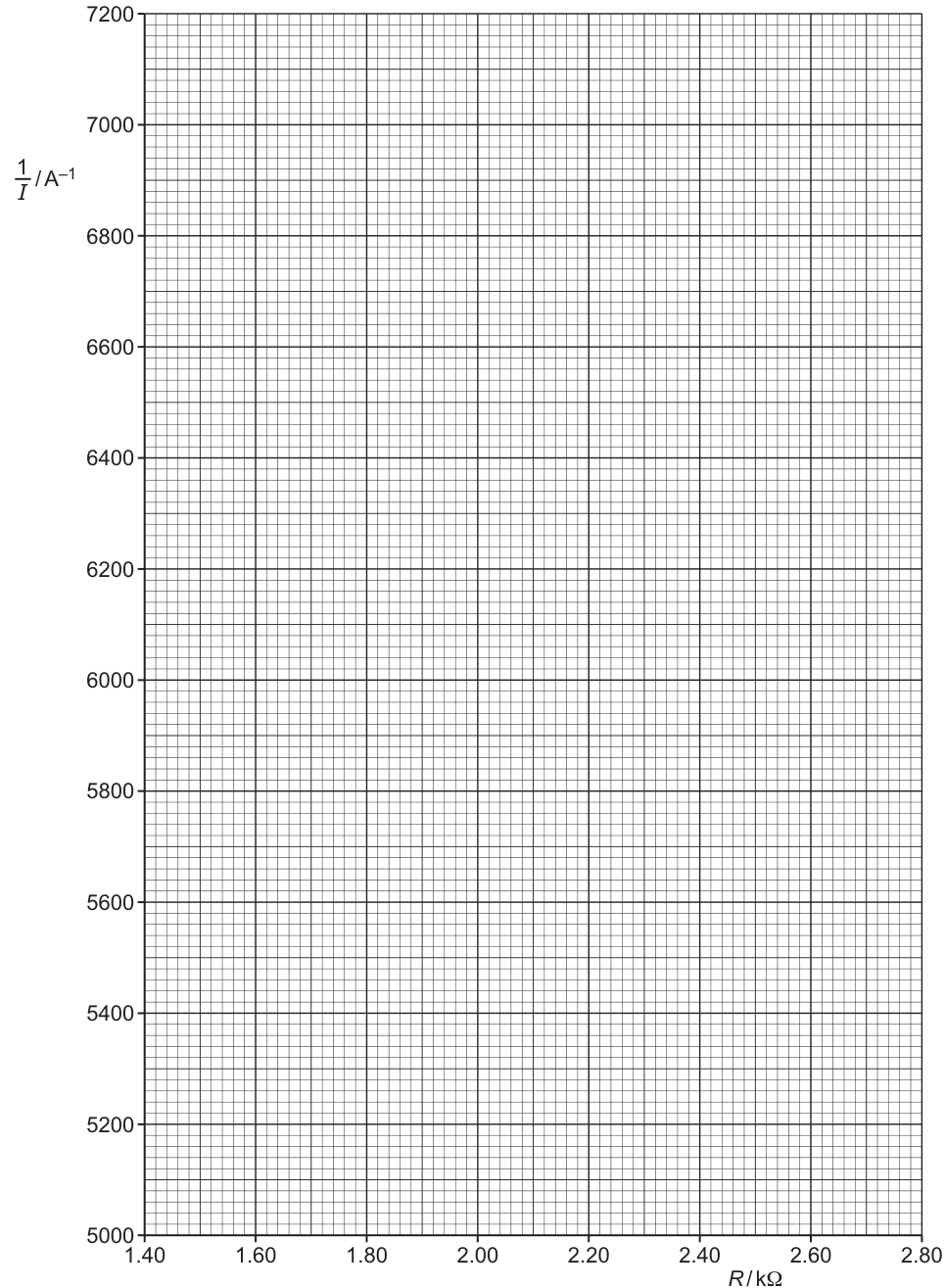
Plot points of against from Table 2.1.
Draw vertical error bars of magnitude for each point.
See graph (points plotted with vertical error bars).
Background Concept
A graph is used to test whether two quantities are linearly related. Experimental uncertainty should be shown using error bars so that later judgments (such as a worst acceptable line) are justified.
In this question:
- is .
- is in .
- Only has uncertainties provided (from ), so only vertical error bars are required.
Understanding the Question
You must transfer your calculated values (and their absolute uncertainties) onto Graph 2.1 by plotting:
- each point,
- an error bar for each point extending up and down by the absolute uncertainty in .
Approach
- Choose a sensible scale (Graph 2.1 is already scaled).
- Plot each point carefully.
- For each point, draw a vertical line centered on the point with total height .
Step-by-Step Reasoning
- Read directly in from the table (e.g. ).
- Use your computed in .
- For each, draw the error bar from
Key Takeaways
- Correct units and labels are essential: and .
- Error bars represent uncertainty and will be used to judge the range of acceptable straight lines.
Common Mistakes
- Plotting instead of .
- Plotting in when the axis is .
- Drawing error bars of incorrect size (e.g. using directly on the axis).
Things to Be Careful About
- Use a sharp pencil and plot points to within half a small square.
- Error bars must be centered on the plotted point and must be vertical (since uncertainties are not given).
Draw the straight line of best fit and a worst acceptable straight line on your graph. Label both lines.
Answer
Draw a straight line of best fit through the plotted points.
Draw a worst acceptable straight line (steepest or shallowest) that still passes through all the error bars.
Label the lines "best fit" and "worst".
See graph (best-fit line and worst acceptable line drawn and labelled).
Background Concept
A best-fit line represents the most likely linear relationship between and . Because data have uncertainty, many straight lines might be consistent with the measurements. A worst acceptable line is chosen to estimate uncertainty in gradient and intercept:
- It must still be consistent with the data within error bars.
- It should be the steepest or shallowest line that is still acceptable.
Understanding the Question
After plotting points with error bars, you must:
- draw the best-fit straight line,
- draw one worst acceptable straight line,
- label both, because later parts use them to calculate uncertainties in gradient and intercept.
Approach
- Best-fit line: balance the points (roughly equal scatter above and below, not forced through the origin unless justified).
- Worst acceptable line: rotate the line to make it as steep (or as shallow) as possible while still intersecting every vertical error bar.
Step-by-Step Reasoning
- Use a ruler to draw the best-fit line through the trend of the points.
- For the worst acceptable line:
- pick two points near the ends of the graph range,
- ensure the line goes through the top of one end error bar and the bottom of the other end error bar (for maximum change in slope),
- check it still intersects all intermediate error bars.
- Label each line clearly on the graph.
Key Takeaways
- Worst acceptable line is defined by error bars, not by how far it is from the best-fit line.
- The uncertainty in gradient/intercept comes from comparing best-fit with worst-fit.
Common Mistakes
- Drawing a second line that does not pass through all error bars.
- Choosing a line that is only slightly different from the best-fit (not truly “worst”).
- Forgetting to label the two lines.
Things to Be Careful About
- Use end points far apart to make gradient calculations reliable.
- Ensure the worst acceptable line is still straight and consistent across the whole data range.
Determine the gradient of the line of best fit. Include the absolute uncertainty in your answer.
gradient = ______
Working
Using two points on the best-fit line (e.g. near the ends):
Example:
Worst acceptable gradient (from worst line) gives about (or shallowest ).
Answer
(1.47 ± 0.12) × 10^3 A^-1 kΩ^-1
Background Concept
For a straight-line graph, the gradient is
To reduce the effect of reading uncertainty, you should use two points far apart on the line (a large triangle). In Paper 5 analysis, uncertainty in gradient is usually estimated using a worst acceptable line:
Understanding the Question
You have drawn:
- a best-fit line,
- a worst acceptable line.
You must find the best-fit gradient and include an absolute uncertainty based on the difference between the gradients of these two lines.
Approach
- Choose two well-separated points on the best-fit line (not necessarily data points).
- Compute .
- Choose two well-separated points on the worst line and compute .
- Uncertainty is the absolute difference.
Step-by-Step Reasoning
- Read two points on the best-fit line, for example near and .
- Calculate:
- Repeat for worst line (using points on that line).
- Then:
This is why part (c)(ii) is important: your chosen worst line controls the uncertainty you obtain.
Key Takeaways
- Use a large triangle for gradients.
- The uncertainty in gradient is obtained by comparison with the worst acceptable line.
Common Mistakes
- Using two nearby points, giving a large percentage error.
- Calculating instead of .
- Taking half the difference between gradients (Cambridge typically expects the full difference here).
Things to Be Careful About
- Keep units as because the -axis is in .
- Ensure you read from the line, not from the plotted points unless they lie exactly on the line.
Determine the -intercept of the line of best fit. Include the absolute uncertainty in your answer.
-intercept = ______
Working
From the best-fit line, -intercept .
From the worst acceptable line, (or ).
Answer
(2.96 ± 0.24) × 10^3 A^-1
Background Concept
For a straight line
the -intercept is the value of when . On a graph, it is where the line crosses the -axis.
Because the line is determined from uncertain data, the intercept also has uncertainty. As with the gradient, Paper 5 commonly estimates this by comparing the best-fit and worst acceptable lines:
Understanding the Question
You must read the intercept of the best-fit line and include an absolute uncertainty. The uncertainty comes from how much the intercept changes when using the worst acceptable line.
Approach
- Extend the best-fit line to the -axis (at ).
- Read the intercept .
- Extend the worst acceptable line to the -axis and read .
- Compute .
Step-by-Step Reasoning
- Even if is not on the grid, you can extrapolate the straight line back to the -axis.
- Read carefully using the grid scale.
- The worst line generally gives either a larger or smaller intercept than the best line.
- Take the difference as the absolute uncertainty.
Key Takeaways
- Intercept is found at .
- Uncertainty is determined by comparing best-fit and worst-fit intercepts.
Common Mistakes
- Reading the intercept at the smallest value instead of at .
- Forgetting to include an uncertainty.
Things to Be Careful About
- Extrapolation should be along the straight line you have drawn (use a ruler).
- Keep units: intercept is in .
Using your answers to (a), (c)(iii) and (c)(iv), determine the values of and . Include appropriate units.
Data:
= ______
= ______
Using (a) with on -axis:
So
With :
Intercept :
With and :
Answer
E = 1.41 V, Z = 3.02 × 10^3 Ω
Background Concept
Once a straight-line graph has been made, the measured gradient and intercept can be matched to theoretical expressions to determine unknown constants.
Here, after linearising, we have
with . From part (a):
These allow you to find first from , then , and finally from .
Understanding the Question
You are given:
- ,
- your measured gradient and intercept from the graph.
You must determine:
- the cell e.m.f. (in V),
- the resistor value (in ).
Approach
- Use to calculate .
- Rearrange to get .
- Use to get .
Step-by-Step Reasoning
From
rearrange:
Substitute your gradient to obtain a numerical value for in volts. Then
so
Finally, from
rearrange:
Note: has units and has units V, so has units , as required.
Key Takeaways
- Gradient gives directly.
- Intercept then gives once is known.
- Dimensional checking confirms the algebra ().
Common Mistakes
- Using (forgetting the factor from ).
- Substituting with the wrong sign.
- Not giving units for and .
Things to Be Careful About
- Ensure your gradient unit matches your formula (because was ).
- Keep consistent significant figures (usually 3 s.f. is acceptable for derived constants).
From (d)(i):
Fractional uncertainty:
With and :
Since
Answer
absolute uncertainty in
0.07 V
Background Concept
Uncertainty propagation rules commonly used at A level:
- For , the fractional uncertainties are equal:
- For , absolute uncertainties add:
- For (division by an exact constant ), the absolute uncertainty scales:
Understanding the Question
You have found using
You are asked for the absolute uncertainty in . The uncertainty in comes from:
- uncertainty in the gradient (from best vs worst line),
- uncertainty in (given as ).
Approach
- Find uncertainty in using fractional uncertainty in .
- Combine with as a sum.
- Divide by 3 to get .
Step-by-Step Reasoning
Because
and is exact (from unit conversion), the fractional uncertainty is
So
Next,
The uncertainty in the numerator is
so
Key Takeaways
- Use fractional uncertainties for inverse relationships.
- Use absolute uncertainty addition for sums.
- Division by an exact number divides the absolute uncertainty by that number.
Common Mistakes
- Adding fractional uncertainties when the relationship is a sum.
- Forgetting to include the uncertainty in .
- Using (that would be a calculus absolute method but must still be applied correctly; the fractional method is simpler here).
Things to Be Careful About
- Make sure and are in the same units.
- Quote the final uncertainty to 1 significant figure (or 2 if it begins with 1 or 2); is appropriate.
The experiment is repeated. Determine the resistance that gives a value of of .
= ______
Using .
For :
Answer
7.1 × 10^2 Ω
Background Concept
Once you have a linear relationship
you can predict the value of needed to produce a desired by rearranging:
In this question, the graph relates to .
Understanding the Question
You are asked for the resistance that would give a current of . Using the straight-line relationship from the graph (your best-fit line), you:
- convert to ,
- use the line equation to find ,
- convert to .
Approach
- Calculate for .
- Substitute into .
- Solve for .
Step-by-Step Reasoning
Compute the reciprocal current:
Now rearrange the line equation:
Substitute the numerical values of and from your best-fit line to obtain , then multiply by to convert to .
Key Takeaways
- A straight-line graph lets you interpolate/extrapolate to find values not directly measured.
- Here, you must convert from current to before using the graph equation.
Common Mistakes
- Using instead of .
- Forgetting that the -axis is in and giving too large by a factor of .
Things to Be Careful About
- Keep consistent significant figures (typically 2 s.f. is fine for a value derived from a graph).
- If your own and differ slightly from the representative values here, your will differ correspondingly; method marks come from correct substitution and rearrangement.