Physics 9702/52 — October/November 2024
Cambridge A-Level · Planning, Analysis and Evaluation · worked solutions for every part, with the mark scheme
Topics Analysis, Conclusions and Evaluation · Planning
Fig. 1.1 shows a coil made from resistance wire.
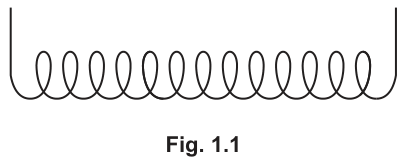
The coil is placed in cooking oil of mass . The total length of the resistance wire in the oil is .
A potential difference is applied to the coil. The temperature of the oil increases by in time .
It is suggested that is related to by the relationship
where is the cross-sectional area of the wire, and and are constants.
Plan a laboratory experiment to test the relationship between and .
Draw a diagram showing the arrangement of your equipment.
Explain how the results could be used to determine values for and .
In your plan you should include:
- the procedure to be followed
- the measurements to be taken
- the control of variables
- the analysis of the data
- any safety precautions to be taken.
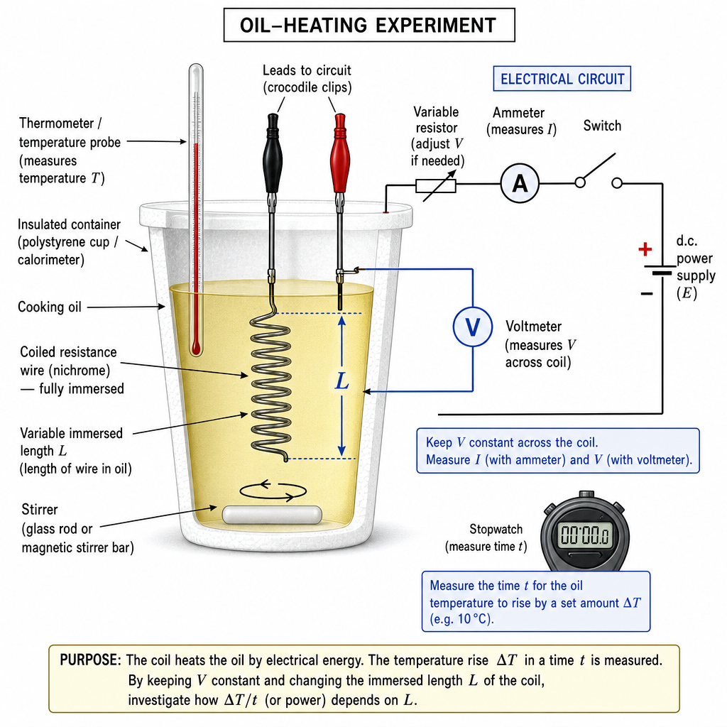
Method (procedure and measurements)
- Put cooking oil in an insulated container (e.g. polystyrene cup / calorimeter) and measure its mass using a balance.
- Immerse a resistance-wire coil fully in the oil. Arrange the wire so the length in the oil can be changed (e.g. marked wire with crocodile clips / adjustable immersion depth). Measure with a metre rule (or measure total immersed length directly).
- Measure wire diameter with a micrometer and calculate
- Connect the coil to a d.c. power supply with a switch. Use a voltmeter across the coil to set and keep constant.
- Place a thermometer/temperature probe in the oil and stir continuously (or use a magnetic stirrer).
- For a chosen , record the initial temperature . Switch on and heat for a fixed time (stopwatch). Switch off and record the final temperature .
- Repeat for at least 5–6 different values of over a wide range. Repeat readings and average .
Control of variables
- Keep constant (same mass of oil each run).
- Keep constant (monitor with voltmeter) and keep constant.
- Use the same wire throughout so is constant.
- Keep initial temperature the same for each run (allow oil to cool back to the same starting temperature).
- Reduce heat loss consistently: lid/insulation, same container, continuous stirring, coil not touching sides.
Analysis to test relationship and find and
- For each run calculate
- Plot a graph of (vertical) against (horizontal).
- If the suggested relationship is correct, the graph is a straight line with
- Gradient so
- -intercept .
Safety
- Hot oil can cause burns: wear eye protection, use a heatproof mat, do not overheat, handle container carefully.
- Electrical safety: use low voltage, keep hands dry, switch off power before adjusting the coil/clips.
See working (plan + graph gives K from gradient and Z from intercept).
Background Concept
The coil is a resistive heater. When a potential difference is applied, electrical energy is transferred to thermal energy in the oil. The temperature rise depends on how much energy is delivered and on the heat capacity of the oil.
The suggested model is
where:
- is the cross-sectional area of the wire (constant if the same wire is used),
- is the heating time,
- is the p.d. across the wire,
- is the length of wire actually in the oil (this affects resistance and hence heating),
- is the oil mass,
- and are constants to be found.
This is already in a linear form: it matches if we define
Then the gradient is and the intercept is .
Understanding the Question
You must propose a practical experiment that changes and measures the resulting temperature rise after a known time at a known p.d. , while keeping other factors (especially , , , and ) controlled.
You also have to explain how to process the measurements so that you can obtain numerical values for and from your results.
Approach
- Choose variables: make the independent variable (you deliberately change it) and measure as the dependent variable.
- Keep key controls fixed: , , , and wire properties () must be constant so that any change in is due to changing .
- Collect a range of readings: take several different values of to allow a meaningful straight-line test.
- Linear analysis: for each reading compute and plot against . Extract and from gradient and intercept.
Step-by-Step Reasoning
- Apparatus set-up
- Put oil in an insulated container to reduce heat losses to the surroundings. Heat loss is a major reason data do not fit a straight line.
- Put the wire coil fully in the oil and ensure it does not touch the container walls (otherwise heat can conduct directly into the container).
- Insert a thermometer/temperature probe and stir continuously so the measured temperature represents the whole oil volume (oil develops temperature gradients if not stirred).
- How to vary and measure
- The key experimental challenge is changing the length of wire in the oil in a controlled, measurable way.
- A practical method is to use a long wire with length marks and crocodile clips so only a chosen section is in circuit and immersed, or to adjust the immersion depth of a marked wire.
- Each time you change , measure it with a ruler/metre rule. You need several values (typically 5–6+) spread over a good range so the graph gradient and intercept are reliable.
- Measurements of , , , and
- Measure on a balance (and keep it constant for all trials).
- Measure with a voltmeter across the coil and adjust the supply so is the same for every run.
- Use a stopwatch to keep constant. Starting and stopping at the right times matters because heating power is continuous.
- Determine by measuring diameter with a micrometer:
Using the same wire ensures is not a changing variable.
- Determining
- Record the initial temperature just before switching on.
- Heat for exactly time , then record the final temperature .
A good control is to begin each trial from the same (let the oil cool back, or use fresh oil at the same starting temperature).
- Data analysis to test the model
- For each trial compute
- Plot (vertical axis) against (horizontal axis). If the model is correct, the points should lie close to a straight line.
- Draw a best-fit straight line.
- Finding and
Comparing
with gives:
- gradient ,
- intercept .
So reading the gradient and intercept from your best-fit line directly provides and .
(If you also draw a worst acceptable line, you can estimate uncertainties in gradient/intercept and hence uncertainties in and .)
Key Takeaways
- In planning questions, marks come from a workable method, clear measurements, and controls.
- Turn the given relationship into a straight-line graph so constants can be read from gradient/intercept.
- Ensure the experiment really varies only the intended independent variable () while keeping , , , and fixed.
Common Mistakes
- Plotting the wrong variables (e.g. vs without linearising/without using the given equation), which prevents and being found.
- Not stating how is changed and measured (you must explain a practical way to vary immersed length).
- Failing to control (assuming the supply setting is constant without measurement).
- Not stirring the oil, leading to unreliable temperature readings.
- Ignoring heat loss and not using insulation/lid, causing poor linearity.
Things to Be Careful About
- Units and consistency: use SI units in calculations ( in , in , in , in , in ).
- Starting temperature: if differs between runs, heat losses to surroundings can differ too, reducing the straight-line quality.
- Electrical heating changes resistance: the wire’s resistance changes with temperature; keeping temperature rises moderate and using a constant helps consistency.
- Avoid superheating oil: keep temperature safely below smoking point and handle hot apparatus carefully.
- Graph quality: use enough points and a wide range of (or ) so gradient and intercept are determined with smaller percentage uncertainty.
A student investigates the refraction of white light entering a transparent rectangular block. A narrow beam of light enters the block at the midpoint of one of the shorter sides. The angle of incidence is measured, as shown in Fig. 2.1.
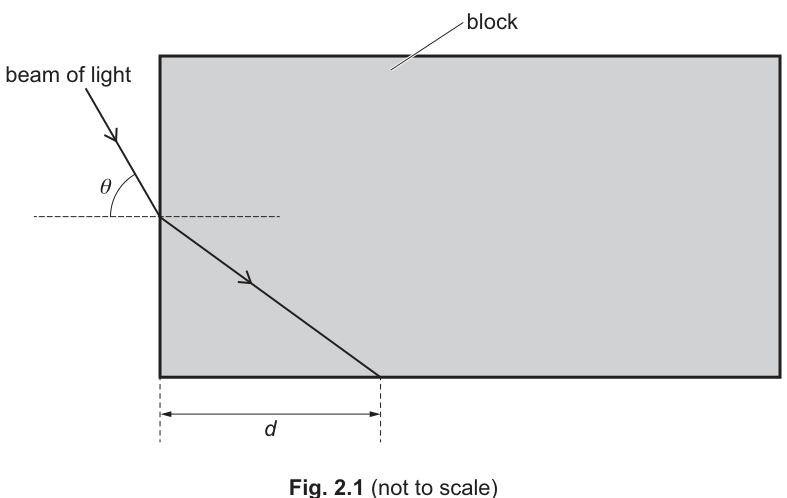
The distance between the corner of the block and the point where the beam of light touches the boundary of the block is measured.
The experiment is repeated for different values of .
It is suggested that and are related by the equation
where and are constants.
A graph is plotted of on the -axis against on the -axis.
Determine expressions for the gradient and -intercept.
gradient = ______
-intercept = ______
Working
Given
Divide by :
So with and ,
Answer
gradient
-intercept
gradient = Bn^2, y-intercept = -B
Background Concept
To use a graph to find constants, we try to rewrite the given relationship into a straight-line form
If we decide what to plot on the axes (here and ), then we rearrange the physics equation until it looks like a constant multiplied by , plus a constant term. The constant multiplying is the gradient , and the constant term is the intercept .
Understanding the Question
You are told that
and that a graph of (vertical axis) against (horizontal axis) is plotted. The task is to express the gradient and the intercept in terms of the constants and .
Approach
- Start with the given equation.
- Rearrange to make the subject.
- Ensure your final expression is in the form
- Read off gradient and intercept by comparison with .
Step-by-Step Reasoning
Start with
Cross-multiply:
Expand the right-hand side:
Make the subject:
Divide by :
Now compare with where and :
- gradient
- intercept
Key Takeaways
- Linearisation means rearranging to match using the chosen axes.
- Gradient is the coefficient of the plotted -quantity.
- Intercept is the constant term (value of when ).
Common Mistakes
- Giving gradient as (from not rearranging fully).
- Missing the negative sign in the intercept.
- Treating the intercept as .
Things to Be Careful About
- The graph uses , not .
- Keep bracket/expansion steps clear so the coefficient of is unambiguous.
Values of , and are given in Table 2.1.
Table 2.1
| 28.5 | 4.39 | ||
| 33.5 | 3.28 | ||
| 42.5 | 2.19 | ||
| 50.0 | 1.70 | ||
| 57.5 | 1.41 | ||
| 63.5 | 1.25 |
Calculate and record values of in Table 2.1.
Include the absolute uncertainties in .
Working
For , absolute uncertainty:
(using ).
- :
- :
- :
- :
- :
- :
Answer
(with absolute uncertainties):
615±10, 458±8.6, 292±6.8, 216±5.9, 166±5.2, 139±4.7 (all in cm^2)
Background Concept
When you calculate a new (derived) quantity from a measured quantity, you should propagate the uncertainty.
Here the derived quantity is
If has absolute uncertainty , then for a power law the fractional uncertainty multiplies by :
For this gives
Understanding the Question
The table gives values, each with . You must:
- calculate for each row;
- calculate the absolute uncertainty in for each row.
These uncertainties are then used as vertical error bars later.
Approach
For each row:
- Compute by squaring.
- Use
- Quote and in .
Step-by-Step Reasoning
Take the first row as an example.
- Measured: .
- Square the central value:
- Propagate uncertainty:
Repeat exactly the same two-step process for each in the table.
Key Takeaways
- For , the absolute uncertainty is .
- Units must be squared too: .
- These uncertainties become the lengths of the graph’s -error bars.
Common Mistakes
- Writing (incorrect for propagation here).
- Forgetting to square the unit.
- Rounding too aggressively so it loses consistency with the uncertainty.
Things to Be Careful About
- Keep the uncertainty to 1–2 significant figures and round to a consistent precision that matches it.
- Use the given for every row (since it is stated constant).
Answer
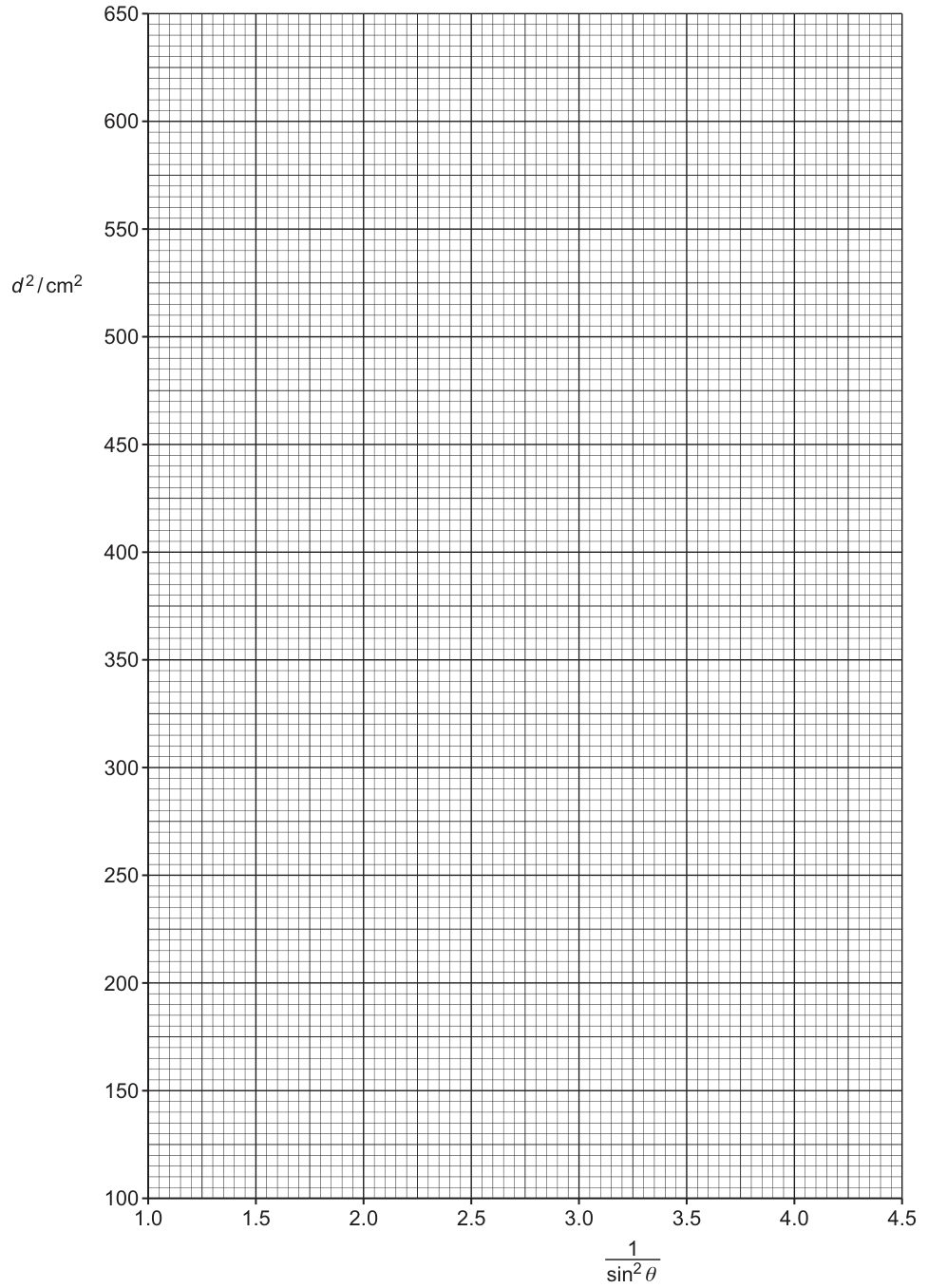
Plot the six points where
with vertical error bars of :
- with
- with
- with
- with
- with
- with
Axes labelled and .
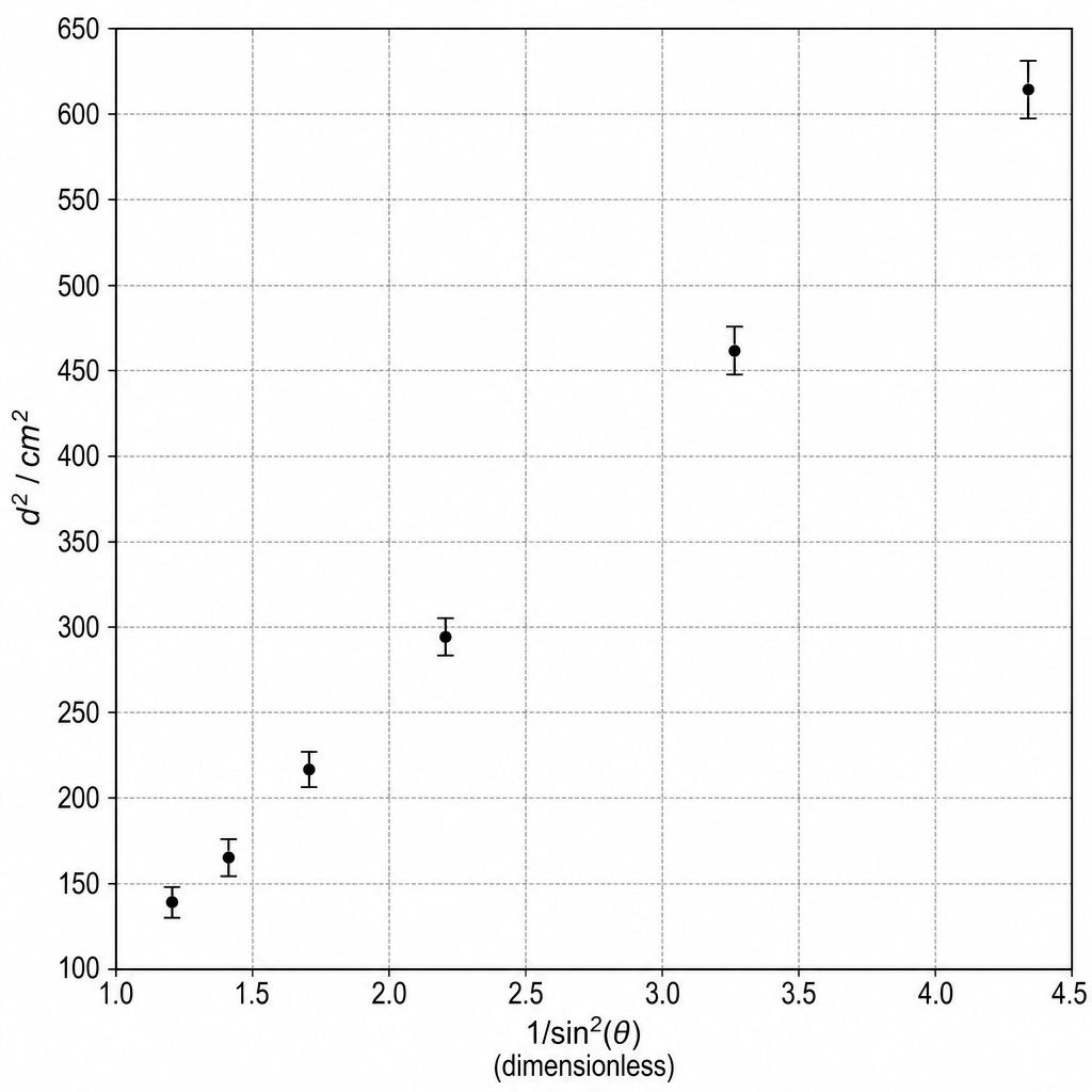
See graph
Background Concept
A good physics graph must:
- have correctly labelled axes (quantity and unit);
- use a sensible scale (use at least half the grid in each direction);
- plot points accurately;
- include error bars when uncertainties are given.
Error bars represent the range within which the true value may lie. Here only (hence ) has an uncertainty provided, so we draw vertical error bars for .
Understanding the Question
You are provided with and you calculated and in part (b). You must place these on the provided grid and show each as a vertical error bar through the point.
Approach
- Put on the horizontal axis and on the vertical axis.
- Choose scales that spread the data out.
- Plot each point.
- For each point, draw a vertical error bar from to .
Step-by-Step Reasoning
- Label axes clearly: on and on (dimensionless).
- Plot the coordinates from the table (six points).
- Add error bars using your computed uncertainties, e.g. for with , the bar runs from to .
Key Takeaways
- Error bars should be centred on each plotted point.
- Only plot error bars for quantities with uncertainties (here, ).
- Clear axis labels and sensible scales are essential for marks.
Common Mistakes
- Missing units on the -axis.
- Drawing error bars horizontally (there is no stated uncertainty in ).
- Using error bar total length instead of .
Things to Be Careful About
- Plotting accuracy: points should be within about half a small square.
- Use the same scale all along each axis; avoid awkward scales that are hard to read accurately.
Draw the straight line of best fit and a worst acceptable straight line on your graph. Label both lines.
Answer
Draw a single straight line of best fit through the trend of the plotted points.
Draw a worst acceptable straight line (steepest or shallowest) that still passes through all the error bars.
Label the lines "best fit" and "worst".
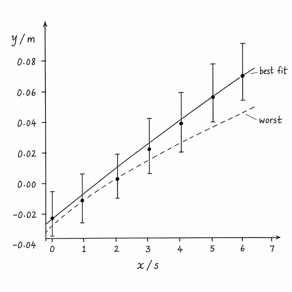
See graph
Background Concept
A best-fit line is drawn to represent the underlying linear relationship, balancing the scatter so that roughly equal numbers of points lie above and below (and the distances are overall minimised).
A worst acceptable line is used to estimate uncertainty in gradient/intercept: it is the steepest or shallowest straight line that is still consistent with the data within their error bars.
Understanding the Question
After plotting points and error bars in (c)(i), you must:
- add the best-fit straight line;
- add one worst acceptable straight line;
- label both, because later parts require gradients and intercepts from them.
Approach
- Draw the best-fit line as a straight line through the middle of the error bars.
- Then try drawing an extreme line (either maximum slope or minimum slope) that still intersects every vertical error bar.
- Choose the extreme that is furthest from the best-fit line (gives the largest difference in gradient/intercept).
Step-by-Step Reasoning
- For the best-fit line: do not join dot-to-dot. Use a ruler and make it a single straight line.
- For the worst acceptable line: rotate the ruler to make the line as steep (or as shallow) as possible, but check it still goes through each error bar range. If it misses even one error bar, it is not acceptable.
Key Takeaways
- Best-fit: "most representative" straight line.
- Worst acceptable: "most extreme" line still consistent with error bars.
- These two lines allow you to estimate uncertainties in gradient and intercept.
Common Mistakes
- Drawing the worst line through the points rather than through the error bars.
- Drawing two worst lines (usually only one is required).
- Forgetting to label the lines.
Things to Be Careful About
- The worst line must remain straight.
- It must intersect all error bars, not necessarily the central points.
- Use long spans on the grid so later gradient measurements are accurate.
Determine the gradient of the line of best fit. Include the absolute uncertainty in your answer.
gradient = ______
Working
Using two well-separated points on the best-fit line, e.g.
Worst acceptable line (example):
Absolute uncertainty:
Answer
(152 ± 5) cm^2
Background Concept
For a straight-line graph of against , the gradient is
To reduce percentage reading error, choose two points that are far apart on the line (large triangle). Do not use two adjacent points.
To estimate uncertainty in gradient in Paper 5, you compare the gradient of your best-fit line with the gradient of a worst acceptable line:
Understanding the Question
You must read the gradient of the best-fit line from your graph and include an absolute uncertainty obtained using the worst acceptable line you drew in (c)(ii).
Approach
- Pick two widely separated points on the best-fit line (they can be convenient grid intersections; they do not have to be original data points).
- Compute .
- Repeat using two points on the worst acceptable line to get .
- Use .
Step-by-Step Reasoning
- Suppose the best-fit line passes close to points like and .
Compute:
So
- From the worst acceptable line, you might obtain a slightly different slope, e.g. .
Uncertainty:
So quote .
Key Takeaways
- Use a large triangle for gradients.
- Uncertainty comes from how much the slope could plausibly change while still fitting within error bars.
Common Mistakes
- Using by accident.
- Using two data points not on the best-fit line (instead of points on the line itself).
- Halving the difference between best and worst gradients (Paper 5 typically uses the full difference).
Things to Be Careful About
- Units: here is dimensionless, so gradient has the same unit as , i.e. .
- Choose points read cleanly from the line to avoid large rounding error.
Determine the -intercept of the line of best fit. Include the absolute uncertainty in your answer.
-intercept = ______
Working
Using with and a point on the best-fit line, e.g. :
Worst acceptable line gives (example):
Absolute uncertainty:
Answer
(-51 ± 10) cm^2
Background Concept
For a straight line
the -intercept is the value of when . On a graph, you can either:
- read it directly by extending the line to the -axis, or
- calculate it using one point on the line and the gradient:
Uncertainty in is estimated similarly to gradient: compare from the best-fit line to from the worst acceptable line.
Understanding the Question
You must find the intercept of the best-fit line on the vs graph and include an absolute uncertainty based on your worst acceptable line.
Approach
- Determine from the best-fit line (direct read-off at , or using ).
- Determine from the worst acceptable line.
- Use
Step-by-Step Reasoning
Using the algebra method with a clearly read point on the best-fit line:
- Suppose .
- Take a point on the best-fit line, e.g. .
Then
Repeat for the worst acceptable line to get a different intercept, e.g. .
So
Key Takeaways
- Intercept can be found by reading at or by .
- Use best vs worst line to estimate intercept uncertainty.
Common Mistakes
- Forgetting that the intercept may be negative.
- Using a point that is not on the drawn best-fit line.
- Quoting an intercept with no unit.
Things to Be Careful About
- Extrapolation to can amplify reading errors; using with a well-chosen point often improves accuracy.
- Units of intercept are the same as (here ).
Using your answers to (a), (c)(iii) and (c)(iv), determine the values of and . Include appropriate units.
= ______
= ______
Working
From (a): gradient and -intercept .
Using -intercept :
Using gradient :
Answer
B = 51 cm^2, n = 1.73
Background Concept
Once you have a straight-line form
you can identify constants in the original physics equation by matching your rearranged expression.
From part (a) we found:
So, if the graph is against :
Also, refractive index is dimensionless.
Understanding the Question
You have numerical values for gradient and intercept from the graph. You must convert these into the constants and using the expressions you derived in (a). You must include appropriate units for .
Approach
- Use to get .
- Use to get .
- Take the square root to find .
- Check units: because has units of , must also be .
Step-by-Step Reasoning
- If the intercept is , then
- If the gradient is , then
- Hence
Key Takeaways
- Intercept gives directly (with a sign change).
- Gradient and together give .
- Units are checked by comparing with the linear equation.
Common Mistakes
- Taking equal to the intercept instead of the negative of the intercept.
- Forgetting to take the square root and giving instead of .
- Giving units for (it is dimensionless).
Things to Be Careful About
- Use consistent significant figures (usually 2–3 s.f. based on graph readings).
- If your intercept is negative, should come out positive (since it represents a squared-length scale here).
Working
So fractional uncertainty:
Using and :
Percentage uncertainty:
Answer
12%
Background Concept
When quantities are multiplied or divided, fractional (or percentage) uncertainties add:
If you then take a power, , the fractional uncertainty multiplies by :
Here
so the factor of appears.
Understanding the Question
You already obtained a value of from the gradient and intercept (giving ). You must now find the percentage uncertainty in , using the uncertainties in and that come from the best and worst acceptable lines.
Approach
- Write in terms of and .
- Write the fractional uncertainty rule for .
- Substitute .
- Convert to percentage.
Step-by-Step Reasoning
Start from
For the inside ratio :
Then applying the square root (power ):
Substitute the values from the graph and evaluate, then multiply by .
Key Takeaways
- Add fractional uncertainties for division.
- Multiply by because is a square root.
- Convert to percentage at the end.
Common Mistakes
- Forgetting the factor .
- Subtracting uncertainties when dividing (they add).
- Using absolute uncertainties directly without first forming fractional uncertainties.
Things to Be Careful About
- Use the uncertainties you obtained from the best vs worst lines (not the scatter of points).
- Keep enough significant figures during intermediate steps so the final percentage is not distorted by rounding.
Working
From (a):
So
Using , , and :
Answer
23.6°
Background Concept
Once constants are found from a linear graph, you can use the model equation to predict values. Here the relationship rearranges to
So if you know , you can solve for and then find using an inverse sine.
Understanding the Question
You repeat the experiment and want the incident angle that would produce a distance . Since is larger than any in the table, you should expect to be smaller than the smallest table value (because smaller gives smaller , larger , hence larger ).
Approach
- Square to get .
- Rearrange the straight-line form to make the subject.
- Invert to get .
- Take the square root to get , then use .
Step-by-Step Reasoning
Start from
Rearrange:
So
Substitute so , and use your graph-derived constants (often easiest is gradient):
Compute , then , then .
Key Takeaways
- Use the straight-line rearranged equation for predictions.
- Using as the gradient avoids carrying separately.
- Check your answer is physically sensible (here should be less than the smallest measured angle).
Common Mistakes
- Using instead of in the equation.
- Forgetting to add to .
- Taking instead of first taking the square root.
Things to Be Careful About
- Calculator mode: ensure degrees.
- Rounding too early can shift by a noticeable amount; keep at least 3 s.f. until the final step.