Physics 9702/51 — October/November 2024
Cambridge A-Level · Planning, Analysis and Evaluation · worked solutions for every part, with the mark scheme
Topics Analysis, Conclusions and Evaluation · Planning
A thin cylindrical bar magnet of length and cross-sectional area is attached to a block. An identical magnet is attached to a trolley, as shown in Fig. 1.1.
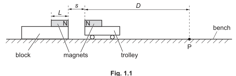
The trolley is held so that the separation of the N poles of the two magnets is .
Point P is a distance from the N pole of the magnet on the stationary trolley.
The trolley is released. The speed of the trolley at point P is determined using one light gate.
It is suggested that is related to by the relationship
where is the magnetic flux density at the N pole of one of the magnets, is the mass of the trolley, and and are constants.
Plan a laboratory experiment to test the relationship between and .
Draw a diagram showing the arrangement of your equipment.
Explain how the results could be used to determine values for and .
In your plan you should include:
● the procedure to be followed
● the measurements to be taken
● the control of variables
● the analysis of the data
● any safety precautions to be taken.
Procedure and measurements
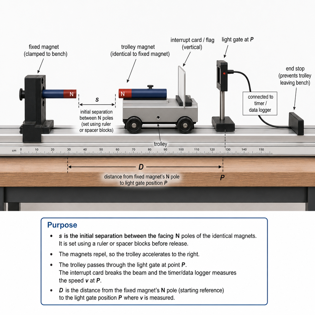
- Set up a low-friction, level track with the fixed magnet rigidly clamped at one end and the second identical magnet on a trolley, with like poles facing.
- Place a light gate at point and connect it to a timer/data logger.
- Attach an interrupt card (flag) of measured length to the trolley.
- Measure and keep constant the distance from the fixed magnet’s N pole to the light gate at .
- Set the initial separation (distance between the two N poles) using a ruler/vernier and spacers; hold the trolley at this position and release it without a push.
- Record the time for the card to pass the light gate and calculate
- Repeat at least 3 times for each and take the mean .
- Change over a wide range (at least 6 values) and repeat.
- Measure of the trolley (balance). Measure and diameter to find (e.g. with calipers, ). Measure at the pole with a Hall probe/teslameter (same position/orientation each time).
Control of variables
- Use the same two magnets throughout (so , , and are constant) and keep temperature similar.
- Keep fixed; keep magnets coaxial and at the same height.
- Ensure track is horizontal; keep friction as constant as possible.
- Use the same release method each time (no initial push).
Analysis (to find and )
From
calculate for each run:
Plot against . A straight line is expected:
Gradient and y-intercept .
Safety
- Keep fingers clear when bringing magnets close (pinch hazard); do not allow magnets to snap together.
- Keep magnets away from sensitive electronics/magnetic media and from people with pacemakers.
- Use an end-stop so the trolley does not run off the bench.
See working
Background Concept
The suggested relationship links the trolley’s speed at a fixed point to the initial separation between the like poles of two identical magnets. The left-hand side
uses the trolley’s kinetic energy term scaled by the fixed distance to point . The right-hand side contains a term proportional to and a constant offset .
A key Paper 5 skill is to test an equation by rearranging it into a straight-line form , so that a graph can be plotted and constants can be obtained from the gradient and intercept.
Understanding the Question
You have:
- two identical bar magnets (length , cross-sectional area ), one fixed, one on a trolley,
- initial separation of the N poles that you can vary,
- a fixed point at distance from the fixed magnet’s N pole,
- a method to measure the trolley’s speed at using one light gate.
You are asked to plan an experiment to test how depends on and to show how to obtain numerical values of the constants and .
Approach
- Choose variables: vary (independent), measure at (dependent), keep and all magnet properties constant.
- Collect data: for each chosen , release the trolley from rest and measure at the light gate.
- Linearise the provided equation by defining
so that plotting vs should give a straight line.
4. Extract constants: use gradient and intercept to determine and .
Step-by-Step Reasoning
1) Setting up and measuring speed
A light gate measures the time for an interrupt card of length to pass through. The instantaneous speed at the gate is then
So you must:
- fix the light gate at point ,
- measure with a ruler/calipers,
- ensure the flag passes cleanly through the gate each time.
2) Choosing values of
You need enough different values to see a trend and produce a meaningful line (typically values). Because the equation involves , small changes in at small separations produce large changes in the force/energy, so:
- use spacers or marked positions to set repeatably,
- measure between the N poles as stated, not between magnet ends or trolley edges.
3) Controlling variables
The equation assumes , , , and are constants.
- : keep the trolley unchanged; measure once with a balance.
- : keep the light gate fixed relative to the fixed magnet’s N pole.
- and : use the same magnets throughout and measure their dimensions.
- : use the same magnet(s) and avoid heating; if measuring with a Hall probe, always measure at the same location/orientation.
- reduce unwanted effects: keep the track level, keep magnets aligned coaxially, and release without pushing.
4) Linearising and plotting
Start from
Define
Then
So a plot of (vertical axis) against (horizontal axis) should give a straight line.
- If the points form a straight line, the relationship is supported.
- If it is not straight, the suggested model is not consistent with the measurements (or controls are poor).
5) Finding and
From the straight-line graph:
- gradient
- intercept
Therefore
and
If uncertainties are required/desired, you would add error bars (notably from and timing) and draw best-fit and worst-acceptable lines to estimate uncertainties in and .
Key Takeaways
- A good plan clearly identifies independent, dependent and controlled variables.
- Use a light gate + interrupt card to measure speed reliably: .
- Turn the given model into a straight-line form by choosing
and . - Determine constants from a graph: gradient gives (after dividing by known factors) and the intercept gives .
Common Mistakes
- Plotting against directly (this will not generally be a straight line).
- Forgetting that the graph intercept is (so is the negative of the intercept).
- Not keeping fixed, or measuring from the wrong point (must be from the fixed magnet’s N pole to the light gate).
- Measuring between the wrong reference points (must be N pole to N pole as defined).
- Releasing the trolley with an extra push, changing the initial kinetic energy.
Things to Be Careful About
- Because , small percentage errors in produce large percentage errors in ; measure as accurately as possible and use a wide range of .
- Ensure the trolley passes the light gate at the same height and without rubbing (otherwise is unreliable).
- Use a large triangle when calculating gradient; do not use two adjacent points.
- Keep magnets aligned; misalignment changes the effective magnetic interaction and makes results scatter.
- Safety: magnets can snap together suddenly and cause injury or damage; also control the trolley motion with an end stop.
A student investigates an electrical circuit. A power supply of electromotive force (e.m.f.) and negligible internal resistance is connected in series to three resistors, each of resistance .
A cell, an ammeter and a resistor of resistance are connected in parallel across one of these resistors, as shown in Fig. 2.1.
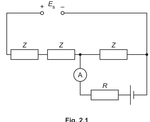
The current is measured by the ammeter for different values of .
It is suggested that and are related by the equation
where is the e.m.f. of the cell.
A graph is plotted of on the -axis against on the -axis.
Determine expressions for the gradient and -intercept.
gradient = ______
y-intercept = ______
Working
From
Answer
gradient
-intercept
gradient = 3/(3E − Es), y-intercept = 2Z/(3E − Es)
Background Concept
To analyse experimental data, we often try to convert a relationship into the straight-line form
where is the gradient and is the -intercept. If we can rewrite the given physics equation so that the measured quantities appear as and , then we can read off expressions for and .
Understanding the Question
You are told the suggested relationship between current and resistance is
A graph is plotted of (vertical axis) against (horizontal axis). So we want an equation of the form
The “something” multiplying is the gradient, and the constant term is the -intercept.
Approach
- Start with the given equation.
- Divide both sides by to make the subject.
- Expand into a term proportional to plus a constant.
- Compare directly with .
Step-by-Step Reasoning
Starting equation:
Divide both sides by :
Now divide by :
Split the fraction into two terms:
Comparing with , with and :
- gradient
- intercept
Key Takeaways
- Linearising means rewriting the physics in form.
- The coefficient of the plotted -quantity is the gradient.
- The constant term is the -intercept.
Common Mistakes
- Leaving the equation as against instead of making the subject.
- Forgetting to split into a term in plus a constant.
- Mixing up the intercept with the gradient.
Things to Be Careful About
- The gradient/intercept expressions depend on what exactly is plotted on the axes. If the horizontal axis is labelled in , a factor of affects the numerical gradient; the algebraic comparison should always reflect the axis units used.
Values of and are given in Table 2.1.
Table 2.1
| 1.50 | ||
| 1.75 | ||
| 1.92 | ||
| 2.22 | ||
| 2.48 | ||
| 2.72 |
Calculate and record values of in Table 2.1.
Include the absolute uncertainties in .
Working
For , fractional uncertainty:
Example (for , ):
Answer
1/I values (A^-1): 5150±53, 5560±62, 5810±68, 6250±78, 6670±89, 6940±96
Background Concept
When you transform data (for example, taking a reciprocal), the uncertainty also changes.
If
then a small change produces a change in of approximately
Equivalently, for reciprocals the fractional (percentage) uncertainty stays the same:
Understanding the Question
You are given current readings in with an absolute uncertainty . You must fill the third column with:
- in (so you must convert to ), and
- the absolute uncertainty in .
Approach
- Convert each current from to , or use the shortcut .
- Compute .
- Find using either:
- , or
- .
- Round the uncertainty sensibly (usually 1 s.f. or 2 s.f.) and round to match.
Step-by-Step Reasoning
Take the first row:
- .
- Reciprocal:
- Uncertainty in the reciprocal:
Using fractional uncertainty,
so
You repeat the same process for each row.
Key Takeaways
- Always ensure units are correct before transforming data.
- For , the fractional uncertainty in equals the fractional uncertainty in .
- Quote in , not .
Common Mistakes
- Calculating using still in without the conversion.
- Writing the uncertainty in as (copying the current uncertainty directly).
- Rounding too aggressively (losing useful precision for plotting).
Things to Be Careful About
- Keep rounding consistent: if the uncertainty is, for example, , then quoting to the nearest unit is unnecessary; nearest is usually fine.
- Uncertainty bars on the graph should use the absolute uncertainty in , not percentage uncertainty.
Answer
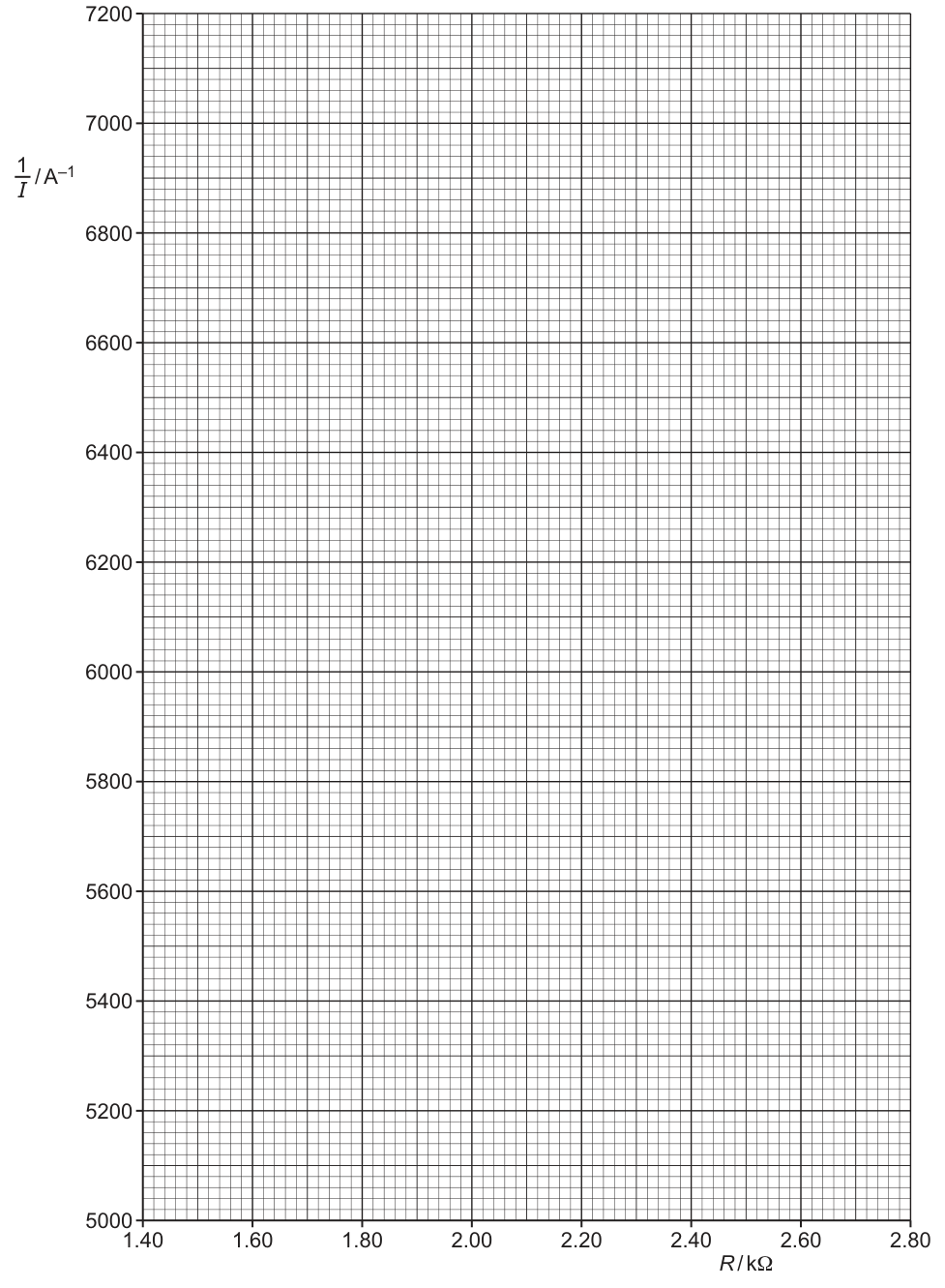
Axes: -axis , -axis .
Plot points:
Draw vertical error bars (in ):
Graph plotted with points and vertical y-error bars for 1/I as calculated.
Background Concept
A good graph in Paper 5 must communicate:
- correct variables on axes with units,
- accurate plotting,
- uncertainties shown as error bars.
Error bars show the range of plausible values of a point. If the uncertainty is only in , the error bars are vertical with half-length equal to the absolute uncertainty in .
Understanding the Question
You have already calculated and its absolute uncertainty for each value of . You must now:
- plot (vertical) against (horizontal), and
- include error bars for .
The provided grid suggests appropriate scales.
Approach
- Check axis labels and units match the instruction: on , on .
- Plot each point carefully.
- For each point, draw a vertical error bar from to .
Step-by-Step Reasoning
- Put values directly on the -axis because the axis is in .
- Use your computed values for the -axis.
- For the first point at , with uncertainty , so the error bar extends from to .
- Repeat similarly for each point.
Key Takeaways
- Error bars must correspond to the calculated absolute uncertainties.
- Axis labels must include both quantity and unit.
- Accurate plotting is essential because gradient and intercept come from the graph.
Common Mistakes
- Drawing error bars with the wrong size (e.g. using instead of converting to in ).
- Missing units on axes.
- Plotting in when the axis is labelled in .
Things to Be Careful About
- Use a sharp pencil and plot to better than half a small square.
- Error bars should be centred on the plotted point.
- Do not force the graph to pass through the origin; you will test that with best-fit/worst-fit lines later.
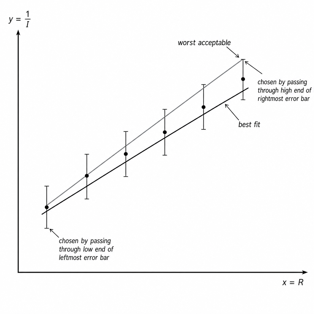
Draw the straight line of best fit and a worst acceptable straight line on your graph. Label both lines.
Answer
Draw a straight line of best fit through the trend of points.
Draw a worst acceptable straight line (steepest or shallowest) that still passes through all the error bars.
Label the lines clearly as “best fit” and “worst acceptable”.
Best-fit and worst acceptable straight lines drawn and labelled.
Background Concept
A line of best fit represents the overall linear trend of the data. Because each point has uncertainty, many straight lines could plausibly represent the relationship.
A “worst acceptable line” is a line chosen to be as different as possible from the best-fit line (usually maximum or minimum gradient) while still being consistent with the data, meaning it passes through (or at least intersects) every error bar.
Understanding the Question
You have plotted vs with vertical error bars. Now you must:
- draw the single straight line that best represents the data trend, and
- draw one additional straight line that is still plausible given the error bars but gives the most extreme gradient.
These two lines will be used in later parts to estimate uncertainties in gradient and intercept.
Approach
- Best-fit line: draw by eye so that points are roughly balanced (similar scatter above and below).
- Worst acceptable line: choose either the steepest or the shallowest line that still intersects every error bar.
- Label both lines on the graph.
Step-by-Step Reasoning
- Start with the best-fit line: it should follow the middle of the vertical spread of the points.
- To get a worst acceptable line, use the end points of the data range:
- for a steep line, aim to go through a low value within the leftmost error bar and a high value within the rightmost error bar;
- for a shallow line, aim to go through a high value within the leftmost error bar and a low value within the rightmost error bar.
- After drawing, check that your worst acceptable line still intersects every error bar. If it misses any, adjust.
Key Takeaways
- Best-fit: balanced through the scatter.
- Worst acceptable: extreme gradient but still consistent with all error bars.
- These two lines are the standard Paper 5 method for gradient/intercept uncertainty.
Common Mistakes
- Drawing the worst line through the outermost plotted points but missing some error bars.
- Drawing two best-fit lines (not making the second one “worst”).
- Forgetting to label which line is which.
Things to Be Careful About
- The worst acceptable line should be a straight line, not a curve.
- Use the full length of the graph when drawing lines to reduce reading error.
- The “worst” line is not chosen randomly; it must be justified by the error bars.
Determine the gradient of the line of best fit. Include the absolute uncertainty in your answer.
gradient = ______
Working
Using two points on the best-fit line (well separated), e.g.
Worst acceptable gradients (from worst line):
So
Answer
(1.48 ± 0.14) × 10^3 A^-1 kΩ^-1
Background Concept
For a straight-line graph, the gradient is
To reduce percentage reading error, you choose two points that are far apart on the line (not necessarily your raw data points, but points on the drawn line).
In Paper 5, the uncertainty in gradient is commonly found by comparing the best-fit gradient with the gradient of a worst acceptable line:
using the worst line that gives the largest difference.
Understanding the Question
You must find:
- the gradient of the best-fit line on your vs graph, and
- an absolute uncertainty in this gradient, using your worst acceptable line.
Approach
- Read two well-separated points on the best-fit line.
- Compute .
- Repeat for the worst acceptable line to find an extreme gradient ( or ).
- Take the absolute difference from the best-fit gradient as the uncertainty.
Step-by-Step Reasoning
- Pick two points on the best-fit line that are near the ends of the plotted range (this makes large).
- Subtract to find and and divide.
- Check units: is in and is in , so gradient unit is .
- For the uncertainty, do the same calculation using the worst acceptable line. If you drew the steepest worst line, that gives ; if you drew the shallowest, that gives .
- The uncertainty is the larger difference between and whichever extreme you found.
Key Takeaways
- Use a large triangle on the line to reduce reading error.
- Always calculate gradient as .
- Worst acceptable line provides an experimental uncertainty estimate.
Common Mistakes
- Using two nearby points so is small (gives a very uncertain gradient).
- Calculating by accident.
- Using raw data points rather than points on the drawn line (the mark scheme expects a line-based gradient).
Things to Be Careful About
- Make sure uses the same axis units you plotted (here ).
- Quote an absolute uncertainty (same units as the gradient), not a percentage, unless asked.
- Keep the number of significant figures sensible: uncertainty typically to 1 s.f. and value to match.
Determine the -intercept of the line of best fit. Include the absolute uncertainty in your answer.
-intercept = ______
Working
From best-fit line, using a point on the line (e.g. , ) and :
Worst acceptable intercepts (from worst line):
So
Answer
(2.96 ± 0.24) × 10^3 A^-1
Background Concept
For a straight line
the -intercept is the value of when . On a plotted graph you can find it by extending the line to cross the -axis.
You can also calculate it from any point on the line:
The uncertainty in the intercept is estimated by comparing the best-fit intercept with the intercept from the worst acceptable line.
Understanding the Question
You must determine the -intercept of your best-fit line on the graph of against , and include an absolute uncertainty based on your worst acceptable line.
Approach
- Find for the best-fit line either by reading at or calculating .
- Find for the worst acceptable line in the same way.
- Uncertainty is the absolute difference between best and worst values (take the larger difference if you have both extremes).
Step-by-Step Reasoning
- Because extrapolating to can be hard to read accurately, using from a clear point on the line is often more accurate.
- Choose a point on the best-fit line that lies exactly on grid intersections if possible.
- Substitute into .
- Repeat using a point on the worst acceptable line to get .
- Compute
Key Takeaways
- Intercept is the value at .
- is a reliable way to compute intercept.
- Worst acceptable line gives uncertainty in .
Common Mistakes
- Using the intercept from the worst acceptable line as the final answer instead of the best-fit intercept.
- Reading from the graph without extending the line properly.
- Mixing up intercept units; it must be in .
Things to Be Careful About
- Keep consistent units: since is in , do not convert to in unless you also convert .
- Quote uncertainty to 1 s.f. (or 2 s.f.) and the intercept to match that precision.
Using your answers to (a), (c)(iii) and (c)(iv), determine the values of and . Include appropriate units.
Data:
= ______
= ______
Working
From (a):
Since the graph uses on the -axis, the gradient is
So
Using -intercept :
Answer
E = 1.41 V, Z = 3.00 × 10^3 Ω
Background Concept
Once you have a straight-line graph, you can extract constants by comparing your experimental straight-line equation with the theoretical one.
If
then and are measured from the graph. If physics predicts
you can equate coefficients to solve for the constants.
Understanding the Question
You have:
- a best-fit gradient from the graph of vs (with plotted in ),
- a best-fit intercept from the same graph,
- a known supply e.m.f. ,
and you must determine the cell e.m.f. and the resistor value .
Approach
- Start from the linear form from (a).
- Adjust the gradient expression to match the fact that is plotted in (this introduces a factor of ).
- Use the measured gradient to find .
- Use to find .
- Use the intercept to find .
Step-by-Step Reasoning
From (a):
If the horizontal axis used in , then gradient would be . But the actual plotted is , i.e. .
Substitute :
So the gradient read from your graph is
Rearrange:
Then use to get :
For , the intercept is still
so
Because is in and in V, their product has units , as expected.
Key Takeaways
- Always match the algebra to the axis units (here introduces a factor ).
- Gradient gives , then follows using the known .
- Intercept gives once is known.
Common Mistakes
- Forgetting the factor from plotting in , which makes wrong.
- Using instead of .
- Giving in without stating the unit, or mixing and inconsistently.
Things to Be Careful About
- Keep enough significant figures in intermediate steps (especially ) before rounding.
- Check unit consistency: if you use in , then you must use (not ) in the formula.
Working
With :
For , absolute uncertainties add in the numerator:
Answer
absolute uncertainty in
0.08 V
Background Concept
Uncertainty rules used here:
- For a reciprocal (or more generally ), fractional uncertainties add:
which can be rearranged to
- For addition/subtraction (), absolute uncertainties add:
- For division by a constant (), absolute uncertainty scales the same way:
Understanding the Question
You already found in (d)(i). Now you must find the absolute uncertainty in .
depends on:
- the measured gradient (with its uncertainty from worst line), and
- the given supply e.m.f. (with uncertainty ).
Approach
- Express in terms of .
- Find the uncertainty in due to uncertainty in .
- Use the relationship between , and , and add absolute uncertainties in the numerator.
Step-by-Step Reasoning
From the graph with in :
Differentiate/uncertainty-propagate for :
Then
Since the numerator is a sum, the absolute uncertainty in the numerator is
Finally divide by 3 to get .
Key Takeaways
- Reciprocal relationships amplify uncertainty when the denominator is uncertain.
- For sums, add absolute uncertainties.
- Dividing by 3 reduces the absolute uncertainty by a factor of 3.
Common Mistakes
- Adding percentage uncertainties when the quantities are being added (should add absolute uncertainties for addition).
- Forgetting to divide the final uncertainty by 3 when calculating .
- Using the intercept uncertainty instead of the gradient uncertainty (here depends on and ).
Things to Be Careful About
- Use in the correct units corresponding to the axis, otherwise is not valid.
- Round uncertainties sensibly; typically 1 s.f. is acceptable for the final absolute uncertainty.
The experiment is repeated. Determine the resistance that gives a value of of .
= ______
Working
Using
With , , :
Answer
705 Ω
Background Concept
Once you have determined constants from a calibration graph (here and ), you can use the original relationship to predict what value of an input (here ) will produce a desired output (here ).
The key skill is rearranging the equation correctly and keeping units consistent.
Understanding the Question
You repeat the experiment and want . Using the same circuit constants (, , and known ), you must find the required resistance .
Approach
- Start from
- Make the subject.
- Substitute converted into amperes.
Step-by-Step Reasoning
Rearrange:
so
and
Convert the target current:
Substitute values (using your earlier best estimates of and ) to obtain .
Key Takeaways
- Always convert to before substituting into equations with volts and ohms.
- Rearranging carefully avoids sign errors.
- A larger current here requires a smaller (a useful reasonableness check).
Common Mistakes
- Substituting instead of .
- Forgetting the factor 3 in .
- Using in while other quantities are in SI units, without conversion.
Things to Be Careful About
- Keep enough significant figures in and before the final rounding.
- Check the answer magnitude: it should be below the earlier range (1.5 to 2.7 k) because is larger than the earlier currents.