Physics 9702/53 — May/June 2024
Cambridge A-Level · Planning, Analysis and Evaluation · worked solutions for every part, with the mark scheme
Topics Analysis, Conclusions and Evaluation · Planning
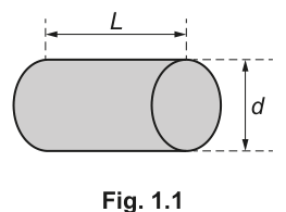
Fig. 1.1 shows a small solid metal cylinder of mass , length and diameter .
The cylinder is heated to a uniform temperature. The cylinder is then removed from the heat source and the cylinder is wrapped in an insulating material.
The temperature of the room is . At time after the cylinder starts to cool, the surface temperature of the cylinder is .
It is suggested that is related to by the relationship
where is the total surface area of the cylinder, is the specific heat capacity of the metal, and and are constants.
Plan a laboratory experiment to test the relationship between and .
Draw a diagram showing the arrangement of your equipment.
Explain how the results could be used to determine values for and .
In your plan you should include:
- the procedure to be followed
- the measurements to be taken
- the control of variables
- the analysis of the data
- any safety precautions to be taken.
Variables
- Independent variable: time after cooling starts.
- Dependent variable: cylinder surface temperature .
- Controlled variables: cylinder dimensions () and material (so fixed), mass , thickness/type of insulation, position of temperature sensor, ambient conditions (air flow, room temperature ).
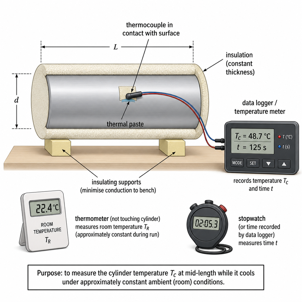
Procedure and measurements
- Measure mass of the cylinder using a balance.
- Measure and using vernier calipers / micrometer.
- Calculate total surface area
- Measure room temperature using a thermometer placed near the apparatus.
- Attach a thermocouple/temperature probe to the cylinder surface (same position each run) using thermal paste and tape.
- Heat the cylinder in a hot water bath (near ) for sufficient time so the temperature is uniform (wait until probe reading is steady).
- Remove cylinder using tongs, quickly wrap with the insulating material (same thickness each run) with the probe still in contact, start timer at the moment of wrapping.
- Record at regular time intervals (or continuously with a data logger) until is close to .
- Repeat the cooling run and average values at each (or repeat the whole run to check repeatability).
Control of variables
- Use the same cylinder throughout (same , , , and material same ).
- Keep insulation type/thickness and wrapping method the same.
- Keep the sensor position and contact method identical.
- Minimise drafts (same location, away from fans/air-conditioning); keep monitored and approximately constant.
- Use the same initial heating condition (e.g. same water-bath temperature and same time immersed).
Analysis of data (to test relationship and find and )
Given
Take natural logs:
- For each reading, calculate and then .
- Plot (y-axis) against (x-axis).
- A straight line supports the suggested relationship.
- Gradient of the line:
- Intercept :
Safety
- Hot cylinder / hot water: use tongs and heatproof gloves; avoid splashing; wear eye protection.
- Keep electrical equipment (data logger) away from water; dry hands before handling plugs/leads.
- Ensure cylinder is placed securely to avoid rolling/falling while hot.
See working
Background Concept
This experiment is based on Newton’s law of cooling, where the rate of energy loss from a hot object is proportional to the temperature difference between the object and its surroundings.
For a body of mass and specific heat capacity , a small temperature drop corresponds to an energy change
If heat is lost from the surface to the surroundings at a rate proportional to surface area and to , then a typical model is
where is an overall heat-transfer coefficient (it depends on insulation, convection, etc.). Solving this differential equation gives an exponential decay:
where is a constant set by the initial conditions (essentially the initial temperature difference at ).
Understanding the Question
You are told a suggested relationship between the cylinder’s surface temperature and time as it cools in a room at temperature .
You must:
- plan a practical method to measure as a function of ,
- ensure the geometry is known to find the surface area ,
- keep other factors constant so the model can be fairly tested,
- show how to process the data to check whether the relationship is exponential,
- and explain how and can be obtained from the results.
Approach
- Choose a reliable way to measure surface temperature continuously: a thermocouple or temperature probe with a data logger gives many readings quickly and reduces reaction-time error.
- Ensure the cylinder starts at a uniform temperature (heat long enough in a well-defined environment such as a hot water bath).
- Wrap in the same insulation each time to keep the heat-transfer conditions (hence ) constant.
- Record and time as it cools, and also measure .
- Linearise the exponential by taking natural logarithms so you can use a straight-line graph. From the gradient and intercept you can find and .
Step-by-Step Reasoning
1) Measuring the required quantities
- Mass : measured with a balance (needed in the exponent).
- Dimensions and : measured with vernier calipers / micrometer. You then compute total surface area:
- Room temperature : measure near the cylinder and keep monitoring; it must be approximately constant for the model.
- Surface temperature : attach a thermocouple firmly to the surface. Good thermal contact matters; use thermal paste and tape.
- Time : start timing at a clearly defined moment (e.g. immediately when wrapping is complete / when removed from bath and wrapped). Use a data logger clock or a stopwatch.
2) Setting up so the model is valid
The model assumes a single, well-defined temperature for the cylinder at each time (or at least that your measured surface temperature is representative). To get close to this:
- heat the cylinder until the temperature is uniform (wait for a steady sensor reading while in the bath),
- keep insulation constant so the cooling conditions don’t change between runs,
- reduce extra heat-loss paths (e.g. do not place the hot cylinder directly on a metal bench; suspend it or place it on insulating supports).
3) Collecting data
Record at equal intervals (e.g. every 10 s) or continuously (best). Continue until is close to because then becomes small and the log values become sensitive to measurement noise; you still want enough data points to see the trend clearly.
Repeat the run to check repeatability. If repeated runs give similar graphs/gradients, that supports that your control of conditions is good.
4) Linearising and extracting and
Start with
Taking natural logarithms gives
This is in the straight-line form with:
- ,
- ,
- intercept ,
- gradient .
So:
and
A straight line on the vs graph is the test of the relationship.
5) Uncertainties (how you would handle them)
- uncertainty comes from probe resolution and imperfect contact; this affects and therefore the log values.
- For the straight-line fit, you can estimate uncertainty in the gradient using a worst acceptable line. Then propagate to using
If is not assumed known, you would include as well.
Key Takeaways
- Exponential relationships are tested efficiently by taking logs to produce a straight-line graph.
- In cooling experiments, controlling heat-transfer conditions (insulation, airflow, contact points) is crucial because they directly affect the constant .
- Gradient and intercept of a linear graph can be mapped to physical constants ( and here).
Common Mistakes
- Plotting against and expecting a straight line (the straight line comes after taking ).
- Forgetting to measure , or assuming it is constant without checking.
- Using the wrong surface area (e.g. only curved surface, or wrong end area).
- Poor thermal contact of the sensor (measures air temperature or insulation temperature instead of the metal surface).
- Changing insulation thickness or wrapping style between runs, which changes .
Things to Be Careful About
- You can only take when ; once is very close to , the difference becomes noisy and logs become unreliable.
- Define clearly and use the same definition for all data.
- Ensure units are consistent when calculating from (use SI: in , in , in , so comes out in ).
- If the cylinder is placed on a surface, conduction into the support adds an extra heat-loss mechanism; this can spoil the simple model unless kept constant and small.
A student investigates the sound from a horn attached to a car, as shown in Fig. 2.1.
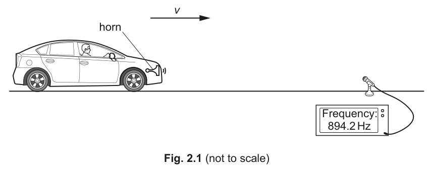
A microphone is placed at the side of the road and connected to a frequency meter. The car travels towards the microphone. The frequency of the sound detected by the microphone is read from the frequency meter.
The speed of the car is measured by two speed detectors. The two measurements of speed are and . The average speed of the car is determined from and .
The experiment is repeated for different speeds of the car.
It is suggested that and are related by the equation
where is the frequency of the sound emitted by the horn and is a constant.
A graph is plotted of on the -axis against on the -axis.
Determine expressions for the gradient and -intercept.
gradient = ______
y-intercept = ______
Working
Given
Take reciprocal:
Comparing with for a plot of against :
Answer
gradient
y-intercept
gradient = -1/(f_s k), y-intercept = 1/f_s
Background Concept
To extract constants from experimental data, a common technique is to rearrange a relationship into the straight-line form
If you plot against , then:
- the gradient (slope) is
- the y-intercept is
This lets you identify unknown constants by comparing your rearranged equation term-by-term with .
Understanding the Question
You are given a suggested relationship between measured frequency and car speed :
A graph is plotted with on the y-axis and on the x-axis. The task is to express this in the form
Then you can read off the gradient and y-intercept.
Approach
- Take the reciprocal of the given equation to create .
- Expand/simplify so it looks like a constant term plus a term proportional to .
- Compare with .
Step-by-Step Reasoning
Starting from
Reciprocal both sides:
Split the fraction:
Simplify :
Now compare with where and :
- gradient
- intercept
Key Takeaways
- Linearise by rearranging into .
- The coefficient of becomes the gradient.
- The constant term becomes the y-intercept.
Common Mistakes
- Forgetting the negative sign in the gradient.
- Stopping at without splitting into constant and terms.
- Mixing up which axis is and which is .
Things to Be Careful About
- The gradient is negative because decreases as increases (since increases).
- Keep and as symbols; do not substitute numbers in part (a).
Values of , and are given in Table 2.1.
Table 2.1
| 3.1 | 3.9 | 894.2 | ||
| 6.7 | 5.9 | 901.2 | ||
| 9.2 | 8.2 | 908.0 | ||
| 11.9 | 10.9 | 915.8 | ||
| 13.3 | 14.5 | 923.6 | ||
| 15.6 | 16.8 | 931.2 |
Calculate and record values of and in Table 2.1.
Include the absolute uncertainties in .
Working
For each run:
Absolute uncertainty in from two readings:
Also
Calculated values:
| 3.1 | 3.9 | 3.5 | 0.4 | 894.2 | 1.118 |
| 6.7 | 5.9 | 6.3 | 0.4 | 901.2 | 1.110 |
| 9.2 | 8.2 | 8.7 | 0.5 | 908.0 | 1.101 |
| 11.9 | 10.9 | 11.4 | 0.5 | 915.8 | 1.092 |
| 13.3 | 14.5 | 13.9 | 0.6 | 923.6 | 1.083 |
| 15.6 | 16.8 | 16.2 | 0.6 | 931.2 | 1.074 |
Answer
and values as in the completed table (with shown for each row).
Completed Table 2.1 values for v, 1/f (×10^-3 Hz^-1), and Δv as shown.
Background Concept
When you have two measurements of the same quantity, a common best estimate is the mean:
A simple absolute uncertainty estimate from the spread of two readings is half the range:
For reciprocals, remember
has units of , and if the table heading is “”, then you should scale by :
Understanding the Question
You are given , (two speed detector readings) and for several runs.
You must fill in:
- the average speed for each run,
- the value of expressed in units of ,
- and include absolute uncertainties in .
Approach
For each row:
- Compute the mean speed .
- Compute the uncertainty using half the difference: .
- Compute and apply the scaling by multiplying by .
- Round sensibly and consistently within each column.
Step-by-Step Reasoning
Example (first row):
Mean speed:
Uncertainty:
Reciprocal frequency with scaling:
So in the table column “” you record .
Repeat this for each row, keeping a consistent decimal place pattern (e.g. to 0.1 , to 0.1 , and to 0.001 in the scaled units).
Key Takeaways
- Mean of two readings gives a best estimate.
- Half the range of two readings is a simple absolute uncertainty.
- Always follow the scaling in the table heading (here ).
Common Mistakes
- Using instead of for the uncertainty.
- Forgetting the scaling and writing instead of .
- Inconsistent rounding/decimal places within a column.
Things to Be Careful About
- Uncertainty should be positive and in the same unit as .
- Check calculator mode for reciprocals; a small slip in powers of ten loses marks.
- The table heading indicates the expected magnitude and rounding.
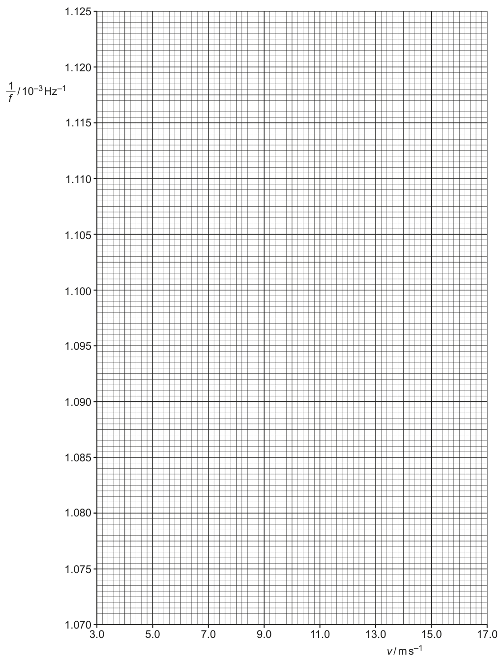
Answer
Plot the points (with in ):
, , , , , .
Include horizontal error bars on each point of size :
, , , , , respectively.
See graph: points plotted with horizontal error bars ±Δv.
Background Concept
A graph is used to reveal trends and allow a best-fit line to be drawn. For experimental work, it is essential to:
- label axes correctly with quantity and unit,
- use a sensible scale that fills much of the grid,
- plot points accurately,
- include error bars when uncertainties are known.
Error bars show the range of values that a measured quantity could reasonably take. Here the uncertainty is in , so the error bars are horizontal.
Understanding the Question
You must plot on the y-axis against on the x-axis, using the values you calculated in Table 2.1.
You must also include error bars for using the absolute uncertainties you found in part (b).
Approach
- Choose appropriate scales (already suggested by the grid provided).
- Plot each coordinate .
- For each point, draw a horizontal error bar from to .
Step-by-Step Reasoning
- Read each and value from your completed table.
- Plot each point as a small cross or dot.
- For row 1, with , so the error bar extends from to .
- Repeat for all points.
The y-values have no stated uncertainty here, so do not draw vertical error bars unless instructed.
Key Takeaways
- Error bars must match the uncertainty and the axis variable.
- Use horizontal error bars when uncertainty is in the x-variable.
Common Mistakes
- Drawing vertical error bars instead of horizontal ones.
- Plotting instead of .
- Ignoring the scaling and plotting values near rather than around .
Things to Be Careful About
- Place points carefully (use half-squares if appropriate).
- Error bars should be centred on the plotted point and have clear end caps.
- Ensure axis labels exactly match those requested on the paper.
Draw the straight line of best fit and a worst acceptable straight line on your graph. Label both lines.
Answer
Draw and label:
- a straight line of best fit through the trend of the plotted points,
- a worst acceptable straight line (steepest or shallowest) that still passes through all the error bars.
Label the lines clearly as “best fit” and “worst acceptable”.
See graph: best-fit line and labelled worst acceptable line drawn.
Background Concept
A best-fit line represents the overall trend of the data, balancing the scatter of points. A worst acceptable line is used to estimate uncertainty in gradient/intercept:
- It must be a straight line.
- It must still be consistent with the data uncertainties (i.e. it passes through all error bars).
- It is chosen to make the gradient (or intercept) as different as possible from the best-fit value.
Understanding the Question
After plotting points with horizontal error bars (uncertainty in ), you must:
- Draw a best-fit straight line.
- Draw one additional straight line that is still acceptable given the error bars, but gives an extreme gradient.
Both must be labelled.
Approach
- Best-fit: draw a line that has roughly equal numbers of points above and below, following the linear trend.
- Worst acceptable: pivot the line to be as steep as possible (or as shallow as possible) while still intersecting every error bar range.
Step-by-Step Reasoning
- Use a ruler to draw the best-fit line through the central trend (not point-to-point zigzags).
- Decide whether a steeper or shallower line would be further from your best-fit gradient.
- Adjust the extreme line until it is just consistent with the error bars. If it misses any error bar region, it is not acceptable.
- Label each line directly on the graph.
Key Takeaways
- Best-fit line: represents trend.
- Worst acceptable line: used to find gradient/intercept uncertainty.
Common Mistakes
- Drawing the worst line through points but ignoring the error bars.
- Drawing a curve instead of a straight line.
- Forgetting to label the two lines.
Things to Be Careful About
- The worst acceptable line must be a single straight line.
- It must pass through all error bars (not necessarily all plotted points exactly).
- Use a sharp pencil/ruler so gradients can be read accurately.
Determine the gradient of the line of best fit. Include the absolute uncertainty in your answer.
gradient = ______
Working
Using large triangles on the best-fit and worst acceptable lines:
Best-fit gradient (from the plotted graph)
Worst acceptable gradient
Absolute uncertainty
Answer
m = (−0.00350 ± 0.00029) (10^−3 Hz^−1) (m s^−1)^−1
Background Concept
The gradient of a straight line is
On a plotted graph, you should use two points far apart on the line (not necessarily data points) to reduce percentage reading error.
To estimate uncertainty in gradient experimentally:
- find from the best-fit line,
- find from the worst acceptable line,
- take the absolute difference as the uncertainty:
Understanding the Question
You have drawn a best-fit line and a worst acceptable line on the graph of against . You must calculate the gradient of the best-fit line and include an absolute uncertainty using your worst line.
Approach
- Choose two widely separated points on the best-fit line.
- Calculate .
- Repeat for the worst acceptable line to get .
- Uncertainty: .
Step-by-Step Reasoning
- Read off two points on the best-fit line, ideally near the ends of the drawn line.
- Compute and in the plotted units.
- Divide to get the gradient.
- Do the same for the worst acceptable line.
- The uncertainty is not a percentage here; it is an absolute uncertainty in the same units as the gradient.
Because the y-axis is labelled in , the gradient unit is per .
Key Takeaways
- Use a large triangle for better precision.
- Worst acceptable line gives a realistic uncertainty estimate.
Common Mistakes
- Using two points very close together (large fractional error).
- Calculating gradient as .
- Taking uncertainty as half the difference when the scheme expects the full difference (or vice versa); always follow the question wording/standard method used.
Things to Be Careful About
- Keep consistent units with the axis scaling ( factor on ).
- Quote uncertainty to 1 (or 2) significant figures and match the decimal places of the gradient value.
Determine the -intercept of the line of best fit. Include the absolute uncertainty in your answer.
-intercept = ______
Working
Best-fit y-intercept:
Worst acceptable y-intercept:
Absolute uncertainty:
Answer
c = (1.131 ± 0.003) (10^−3 Hz^−1)
Background Concept
For a straight line graph, the y-intercept is the value of when . Graphically, you can:
- extend the best-fit line to cross the y-axis and read the value,
- do the same for the worst acceptable line,
- estimate uncertainty with
Understanding the Question
You must obtain the y-intercept of the best-fit line on the graph of (in ) against , and include an absolute uncertainty using your worst acceptable line.
Approach
- Extend the best-fit line to .
- Read off .
- Extend the worst acceptable line to .
- Read off .
- Use .
Step-by-Step Reasoning
- Use a ruler to extend the line smoothly to the y-axis.
- Read the y-axis carefully using the provided scale increments.
- Repeat for the worst acceptable line.
- Quote the intercept with uncertainty in the units of the y-axis (here ).
Key Takeaways
- Intercept uncertainty comes from how much the intercept can change while still fitting within error bars.
Common Mistakes
- Reading the intercept from where the line crosses the x-axis (wrong axis).
- Forgetting the factor and writing as just without indicating units.
- Not using the worst line to estimate uncertainty.
Things to Be Careful About
- Ensure you are reading at , not at the left edge of the grid if it doesn’t start at 0.
- Quote uncertainty to an appropriate number of significant figures and match decimal places.
Using your answers to (a), (c)(iii) and (c)(iv), determine the values of and . Include appropriate units.
= ______
= ______
Working
From (a): y-intercept and gradient for a plot of against .
From the graph (using the axis scaling):
Hence
and using :
Answer
f_s = 8.84×10^2 Hz, k = 3.23×10^2 m s^−1
Background Concept
If a graph has the form
and you have already expressed the physics equation in a matching linear form, then the gradient and intercept can be used to determine constants.
Here, after linearisation you have:
So:
- y-intercept
- gradient
Understanding the Question
You must use your measured gradient and intercept (from the graph of against ) to find numerical values of:
- (frequency emitted by the horn)
- (a constant; it should come out with units of speed)
The graph’s y-axis is in , so you must interpret intercept/gradient with that scaling.
Approach
- Convert the intercept value from “ units” into by multiplying by .
- Use .
- Convert the gradient similarly (multiply by ) to get it in .
- Use to solve for .
Step-by-Step Reasoning
From the straight-line form:
So if the intercept read from the plotted scale is in units of , then the actual intercept in SI units is:
Then
For the gradient, if you read in units of , the SI gradient is:
Finally from
rearrange:
The negative signs cancel because is negative, giving a positive .
Key Takeaways
- Intercept gives directly: .
- Gradient then gives .
- Always handle the axis scaling correctly.
Common Mistakes
- Using in “graph units” without multiplying by .
- Dropping the negative sign in and then getting a negative .
- Mixing up which quantity is and which is .
Things to Be Careful About
- Units: must be in , must be in .
- Significant figures should reflect the graph reading precision.
Working
From (a):
So fractional (percentage) uncertainties add:
Using , , , (in the plotted units):
Answer
8.6%
Background Concept
For multiplication/division, uncertainties are combined using fractional (or percentage) uncertainties:
- If , then
- If , then
This is why the “worst acceptable line” is useful: it gives and .
Understanding the Question
You found using the graph parameters (gradient and y-intercept). Now you must find the percentage uncertainty in , using the uncertainties in the gradient and intercept from parts (c)(iii) and (c)(iv).
Approach
- Write in terms of and .
- Add fractional uncertainties.
- Convert to percentage.
Step-by-Step Reasoning
From the linearised equation:
- intercept
- gradient
Eliminate to get in terms of and :
So
Compute each percentage separately, then add.
Typically the gradient uncertainty dominates because the gradient is found from two read-offs and depends strongly on how the line is drawn.
Key Takeaways
- For , percentage uncertainty in is the sum of percentage uncertainties in and .
Common Mistakes
- Subtracting percentage uncertainties instead of adding.
- Using with its negative sign inside the percentage calculation (use ).
- Mixing SI-scaled values with plotted-scale values inconsistently (though here the scale factor cancels if used consistently for both and ).
Things to Be Careful About
- Use the same units/scaling for and (and for and ).
- Round the final percentage uncertainty sensibly (usually to 2 significant figures).
Working
Given
Rearrange:
Using , and :
Answer
33.9 m s^−1
Background Concept
Once a model (equation) is established and its constants are determined, it can be used for prediction by rearranging and substituting values.
For algebraic rearrangement, keep track of which quantities are constants (, here) and which are variables (, ).
Understanding the Question
You repeat the experiment and now measure a frequency . Using your previously determined values of and , you must find what speed would produce this detected frequency according to the model:
Approach
- Rearrange the formula to make the subject.
- Substitute , , and .
- Quote with unit .
Step-by-Step Reasoning
Starting with
Multiply both sides by :
Divide by :
Rearrange for :
Now substitute in the values you found from the graph. Since (approaching source gives higher detected frequency), the bracket is positive and you get a positive speed.
Key Takeaways
- Rearrangement skills let you use a model to predict unmeasured quantities.
- Sense-check: for an approaching car, should be greater than and should be less than .
Common Mistakes
- Algebra slip: writing (missing factor of ).
- Substituting and with wrong powers of ten due to the scaling earlier.
- Forgetting units on the final speed.
Things to Be Careful About
- Ensure stays positive (here ), otherwise the model would predict an unphysical divergence.
- Use consistent significant figures based on and obtained from the graph.