Physics 9702/52 — May/June 2024
Cambridge A-Level · Planning, Analysis and Evaluation · worked solutions for every part, with the mark scheme
Topics Planning · Analysis, Conclusions and Evaluation
A spring is attached to a strong cylindrical magnet of length and cross-sectional area . The magnet is placed on thin card on top of a magnetic sheet on the bench, as shown in Fig. 1.1.
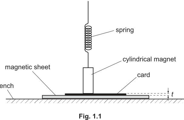
The thickness of the card is . The magnetic flux density at one of the poles of the magnet is .
A force is applied upwards to the spring. The extension of the spring when the magnet just leaves the card is .
It is suggested that is related to by the relationship
where is the spring constant of the spring and is a constant.
Plan a laboratory experiment to test the relationship between and .
Draw a diagram showing the arrangement of your equipment.
Explain how the results could be used to determine a value for .
In your plan you should include:
● the procedure to be followed
● the measurements to be taken
● the control of variables
● the analysis of the data
● any safety precautions to be taken.
Diagram
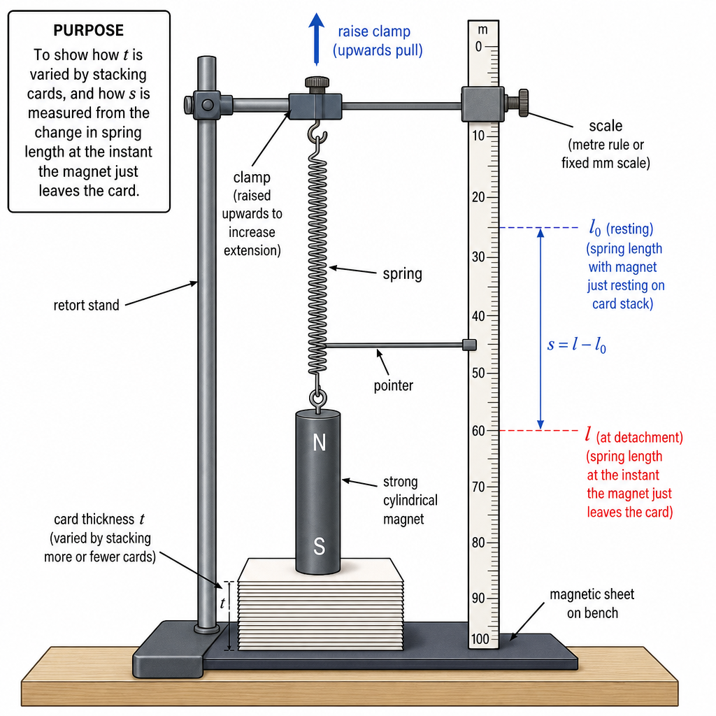
Variables
- Independent variable: total card thickness .
- Dependent variable: spring extension when the magnet just leaves the card.
- Controlled variables: same magnet (fixed , , pole), same spring (fixed ), same magnetic sheet and its position, same orientation and alignment of magnet on the card, same contact area and card material (use identical cards stacked), same temperature.
Apparatus
Retort stand and clamp, spring, cylindrical magnet, magnetic sheet, set of identical thin cards (or card shims) to vary , micrometer screw gauge (or digital calipers) for , metre rule / mm scale fixed next to spring with a pointer attached to the spring or magnet, set square to read the pointer, (optional) camera/phone to judge detachment.
Procedure and measurements
- Set up the magnet attached to the bottom of the vertical spring. Place the magnetic sheet on the bench and place card(s) on top. Put the magnet upright on the card, centred at the same marked position each time.
- Measure the total thickness of the card stack using a micrometer. Take several readings at different points and use the mean.
- With no upward pull, record the spring length (or pointer reading) with the magnet resting on the card.
- Increase the upward pull slowly and steadily (e.g. raise the top clamp in small steps). Identify the instant the magnet just leaves the card (first visible gap / card can be slid freely / video frame where separation begins).
- Record the spring length (or pointer reading) at that instant and calculate the extension
- Repeat steps 3–5 at least three times for the same and calculate the mean .
- Change by adding/removing identical cards to obtain at least 6 values of over a suitable range, and repeat.
Determining
Determine separately by hanging known masses from the spring and measuring extension :
(using a graph of vs ; gradient ).
Analysis of data and determination of
Given
rearrange to
- Calculate for each card thickness.
- Plot a graph of (y-axis) against (x-axis).
- A straight line through the origin supports the relationship.
- Gradient is
so
Safety
- Strong magnet: keep fingers clear to avoid pinching; keep away from phones/computers/credit cards and anyone with a pacemaker.
- Secure the retort stand so it cannot topple; do not overload the spring; keep feet clear if masses are used to determine .
See working
Background Concept
The suggested relationship is
Here is the spring constant (units ), so is a force. The right-hand side must also have units of force, and the relationship predicts an inverse proportionality between the extension at lift-off () and the card thickness ().
To test a relationship experimentally, you vary one variable (independent), measure the response (dependent), keep all other relevant quantities constant (controlled), and then analyse the data in a way that would produce a straight line if the relationship is correct.
A key Paper 5 skill is linearisation. If
then plotting against should give a straight line through the origin. The gradient of that line contains the constant(s) you want, allowing you to determine .
Understanding the Question
You are given an apparatus: a spring attached to a cylindrical magnet resting on card on a magnetic sheet. You pull upwards until the magnet just detaches, and you measure the spring extension at that instant.
You must plan an experiment to check whether changing the card thickness changes according to
You must also explain how to use your results to find . That means your plan must include (i) how to vary and measure , (ii) how to measure reliably at the moment of detachment, (iii) how to measure or know , and (iv) what graph to plot so that can be obtained from a gradient.
Approach
- Choose as the independent variable: use stacks of identical cards so only thickness changes.
- Measure with a micrometer because it is a small thickness.
- For each , slowly increase the extension until the magnet just lifts; record using a fixed scale and pointer to avoid parallax.
- Repeat for each to reduce random uncertainty.
- Determine separately using weights and a force-extension graph.
- Linearise the relationship by plotting vs and use the gradient to calculate .
Step-by-Step Reasoning
1) Setting up and choosing variables
- Independent variable: (easy to vary by adding cards).
- Dependent variable: at the instant of detachment.
- Controlled variables are the quantities appearing in the formula that must not change: , , , , and also practical factors that could change the magnetic interaction (same sheet, same orientation, same position).
2) Measuring thickness well
- A single card may be too thin to measure precisely. Stacking cards increases so the percentage uncertainty in is smaller.
- Use a micrometer to measure total thickness. Take several readings at different points because card can be slightly uneven; average them.
3) Measuring the extension consistently
- You need a clear definition of “just leaves the card”. Good operational definitions include:
- the first moment you can see a gap,
- the card can be slid with negligible friction,
- a video frame where separation begins.
- Record a reference reading with the magnet resting on the card (no upward pull). Then at lift-off record . The extension is
Using a pointer and a fixed vertical scale reduces parallax; reading with a set square helps keep the eye level correct.
4) Repeats
- Detachment is a threshold event and can vary slightly due to small vibrations or how steadily you pull.
- Repeat at least three times for each and take the mean .
5) Measuring the spring constant
You cannot assume unless it is given, so determine it:
- Hang known masses , measure extension .
- Compute force .
- Plot against ; the gradient is because
A graph is better than a single pair of readings because it averages out random error and reveals any non-linearity.
6) Linearising and extracting
Start with
Divide both sides by and rearrange to match :
So if you plot (y-axis) against (x-axis):
- You expect a straight line.
- The line should pass through the origin (within experimental uncertainty) because when (very large ), the model predicts .
- The gradient is
Hence
If , , and are known (or measured separately), then once you have and you can calculate .
Key Takeaways
- A good plan clearly identifies independent, dependent, and controlled variables.
- For an inverse relationship, plotting against the reciprocal of the independent variable is a standard linearisation.
- Threshold measurements (like “just detaches”) require a clear, repeatable criterion and repeats.
- Constants in a model are commonly obtained from the gradient of a straight-line graph.
Common Mistakes
- Plotting against and expecting a straight line (the model predicts , not ).
- Not stating how is obtained, even though is required to find .
- Varying more than one factor at a time (e.g. changing card material as well as thickness, which could change separation, friction, or magnetic properties).
- Measuring with a ruler (insufficient resolution for thin card).
- No clear definition of “just leaves the card”, leading to inconsistent readings.
Things to Be Careful About
- Ensure the magnet is always oriented the same way (same pole toward the sheet) because at the pole could differ if orientation changes.
- Keep the contact area and alignment consistent: always place the magnet at the same marked position on the card and keep it vertical.
- Pull up slowly to reduce overshoot; vibrations can cause premature detachment.
- Use a sufficiently wide range of (and therefore ) to make the graph gradient more reliable.
- Quote and to sensible precision (micrometer resolution for ; mm scale for ) and use mean values from repeats.
- Handle strong magnets safely and keep them away from sensitive devices and medical implants.
A student investigates the resonant frequency of a metal rod. The metal rod of length is suspended from two rubber loops. A sensitive microphone with a cone is positioned at one end of the rod. The microphone is attached to an oscilloscope, as shown in Fig. 2.1.
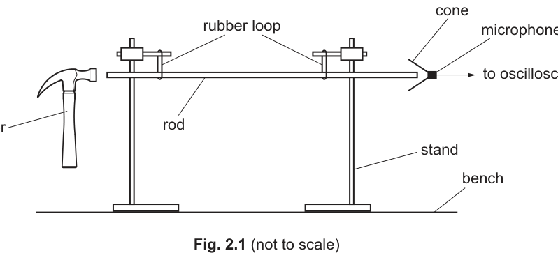
The rod is hit gently with a hammer.
The period of the trace produced on the oscilloscope is determined.
The experiment is repeated for different values of .
It is suggested that and are related by the equation
where and are constants.
A graph is plotted of on the -axis against on the -axis.
Determine expressions for the gradient and -intercept.
gradient = ______
y-intercept = ______
Take (\lg) of
Answer
gradient (= n)
(y)-intercept (= \lg!\left(\frac{2}{C}\right))
gradient = n; y-intercept = lg(2/C)
Background Concept
A power-law relationship can be tested by taking logarithms. If
then taking base-10 logs gives
which is a straight-line form (y = mx + c) with (y = \lg T), (x = \lg L), gradient (m = n) and intercept (c = \lg k).
Understanding the Question
You are told
and that a graph of (\lg T) (vertical axis) against (\lg L) (horizontal axis) is plotted. The question asks what the gradient and the y-intercept represent in terms of the constants (n) and (C).
Approach
- Take (\lg) of both sides.
- Rearrange into (\lg T = (\text{something}),\lg L + (\text{constant})).
- Compare with (y = mx + c).
Step-by-Step Reasoning
Start with
Take (\lg) of both sides:
Use log rules (\lg(ab)=\lg a+\lg b) and (\lg(L^n)=n\lg L):
So for a plot of (\lg T) against (\lg L):
- gradient (= n)
- y-intercept (= \lg(2/C))
Key Takeaways
- Logarithms turn (T \propto L^n) into a straight line.
- The power (n) becomes the gradient on a log-log plot.
- The constant factor becomes the y-intercept (as a log).
Common Mistakes
- Writing the intercept as (\lg(2C)) instead of (\lg(2/C)).
- Forgetting that (\lg(L^n)=n\lg L).
Things to Be Careful About
- The base of the log is (10) because (\lg) is used.
- Keep the linear form clearly as (\lg T = n\lg L + \lg(2/C)) before reading off (m) and (c).
Values of and are given in Table 2.1.
Table 2.1
| 54 | |||
| 70 | |||
| 86 | |||
| 108 | |||
| 140 | |||
| 167 |
Calculate and record values of and in Table 2.1.
Include the absolute uncertainties in .
For (\lg T),
Completed Table 2.1 (logs to 3 d.p.):
| (L/\text{cm}) | (T/10^{-5},\text{s}) | (\lg(L/\text{cm})) | (\lg(T/10^{-5},\text{s})) |
|---|---|---|---|
| 54 | (24\pm1) | (1.732) | (1.380\pm0.018) |
| 70 | (32\pm1) | (1.845) | (1.505\pm0.014) |
| 86 | (39\pm1) | (1.935) | (1.591\pm0.011) |
| 108 | (49\pm2) | (2.033) | (1.690\pm0.018) |
| 140 | (64\pm2) | (2.146) | (1.806\pm0.014) |
| 167 | (74\pm2) | (2.223) | (1.869\pm0.012) |
lgL: 1.732, 1.845, 1.935, 2.033, 2.146, 2.223; lgT: 1.380±0.018, 1.505±0.014, 1.591±0.011, 1.690±0.018, 1.806±0.014, 1.869±0.012
Background Concept
When plotting a log-log graph, you need (\lg) values. If a measured quantity (T) has an absolute uncertainty (\Delta T), the uncertainty in (\lg T) is found from differentiation:
so
This gives an absolute uncertainty in the plotted (y)-value, used for error bars.
Understanding the Question
You are given values of (L) (in cm) and (T) (in units of (10^{-5},\text{s})) with uncertainties in (T). You must:
- calculate (\lg(L/\text{cm})) for each row,
- calculate (\lg(T/10^{-5},\text{s})) for each row,
- include absolute uncertainties in (\lg T) (i.e. in the log values of (T)).
Approach
- Use a calculator to find each (\lg) value.
- For each (T\pm \Delta T), compute (\Delta(\lg T)=0.434(\Delta T/T)).
- Record logs to a consistent number of decimal places (typically 3 d.p. for graphing).
Step-by-Step Reasoning
Example for the first row:
- (T = 24) (in units of (10^{-5},\text{s})), (\Delta T = 1).
Log value:
Uncertainty in log:
So record (1.380\pm0.018).
Repeat the same method for each row; the fractional uncertainty (\Delta T/T) is what matters.
Key Takeaways
- Log values are plotted, so you must also convert uncertainties into log-space.
- For (\lg), use (\Delta(\lg T)=\Delta T/(T\ln 10)).
- Consistent decimal places help accurate graph reading.
Common Mistakes
- Using (\Delta(\lg T)=\lg(\Delta T)) (incorrect).
- Forgetting the factor (\ln 10) (or (0.434)).
- Writing too few decimal places, making graphing and gradients inaccurate.
Things to Be Careful About
- The table uses (T/10^{-5},\text{s}), so you take (\lg) of the numbers shown (24, 32, ...).
- Uncertainty in (\lg T) should be absolute (e.g. (\pm 0.014)), not a percentage.
- Keep rounding sensible: log values typically to 3 d.p.; log-uncertainties often to 2–3 s.f.
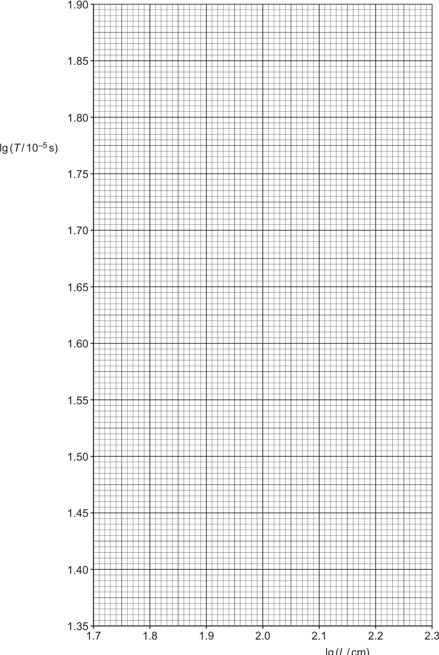
Plot (y=\lg(T/10^{-5},\text{s})) against (x=\lg(L/\text{cm})) with vertical error bars (\pm\Delta(\lg T)).
Points to plot ((x, y)):
- ((1.732,\ 1.380)) with (\pm 0.018)
- ((1.845,\ 1.505)) with (\pm 0.014)
- ((1.935,\ 1.591)) with (\pm 0.011)
- ((2.033,\ 1.690)) with (\pm 0.018)
- ((2.146,\ 1.806)) with (\pm 0.014)
- ((2.223,\ 1.869)) with (\pm 0.012)
See plotted points with error bars (coordinates given in working).
Background Concept
A graph is used to test whether a relationship is linear and to extract constants from the gradient and intercept. When uncertainties are provided for the dependent variable, they must be shown as error bars so that a realistic uncertainty in the gradient/intercept can be estimated.
Understanding the Question
You must plot (\lg(T/10^{-5},\text{s})) (y-axis) against (\lg(L/\text{cm})) (x-axis), using the values you calculated in part (b). You must also include error bars for (\lg T), using the absolute uncertainties (\Delta(\lg T)).
Approach
- Choose sensible scales so the plotted points occupy at least half the grid in each direction.
- Label axes exactly as stated (including the quantity inside the log and the units).
- Plot each point accurately.
- Draw a vertical error bar through each point of total height (2\Delta(\lg T)).
Step-by-Step Reasoning
- Put (x = \lg(L/\text{cm})) on the horizontal axis and (y = \lg(T/10^{-5},\text{s})) on the vertical axis.
- For each row, locate (x) and (y) on the grid and mark a small cross.
- Add the error bar: from (y-\Delta(\lg T)) to (y+\Delta(\lg T)) at that same (x).
For example, the first row is (x=1.732), (y=1.380) and (\Delta y=0.018), so the error bar runs from (1.362) to (1.398).
Key Takeaways
- Correct axis labels and scales are essential marks in Paper 5.
- Error bars must match the uncertainties in the plotted quantity (here, (\lg T)).
Common Mistakes
- Plotting (T) against (L) instead of their logarithms.
- Using error bars based on (\Delta T) rather than (\Delta(\lg T)).
- Omitting units inside the (\lg) label or writing ambiguous labels.
Things to Be Careful About
- Error bars are vertical only here because only (T) uncertainties are given.
- Ensure plotting precision: each point should be within about half a small square of the correct location.
- Use consistent rounding from the table (don’t mix 2 d.p. and 3 d.p. values).
Draw the straight line of best fit and a worst acceptable straight line on your graph. Label both lines.
Draw and label:
- a straight line of best fit through the points,
- a worst acceptable straight line (steepest or shallowest) that still passes within all error bars.
(For example, best-fit may be represented by (y \approx 1.00x - 0.35) and a worst acceptable line by (y \approx 1.06x - 0.47).)
Best-fit line and a labelled worst acceptable line drawn.
Background Concept
A best-fit line represents the most likely linear relationship. To estimate the uncertainty in gradient (and intercept) from experimental scatter and error bars, Paper 5 commonly uses a “worst acceptable line”: the steepest or shallowest straight line that is still consistent with all the plotted error bars.
Understanding the Question
After plotting the data with error bars, you must draw:
- a straight line of best fit (most balanced among the points), and
- one worst acceptable line (either maximum gradient or minimum gradient) that still fits the data within the error bars.
Approach
- Best-fit line: draw a single straight line so that points are roughly equally distributed above and below the line (do not join dots).
- Worst acceptable line: pivot the line to make it as steep or as shallow as possible while still passing through (or at least intersecting) every vertical error bar.
- Label each line clearly (e.g. “best fit” and “worst”).
Step-by-Step Reasoning
- Place a ruler and draw a straight best-fit line through the central trend.
- For the worst line, choose steepest OR shallowest:
- Steepest line: try to go through the bottom of the first error bar and the top of the last error bar (or equivalent extremes), then check all intermediate error bars are still intersected.
- Shallowest line: try to go through the top of the first error bar and bottom of the last error bar, then check again.
- Once you have an acceptable extreme, label it “worst acceptable line”.
Key Takeaways
- Best-fit gives the best estimate of the relationship.
- Worst acceptable line provides an uncertainty estimate in gradient/intercept.
Common Mistakes
- Drawing the worst line that misses one or more error bars (not acceptable).
- Drawing two worst lines when only one is requested, or failing to label them.
- Forcing the best-fit line through the origin without justification.
Things to Be Careful About
- The worst acceptable line must be straight and must be plausible by the error bars, not by the points alone.
- Choose the worst line that gives the greatest difference in gradient from the best-fit line, because that maximises the uncertainty estimate (as required by the method).
Determine the gradient of the line of best fit. Include the absolute uncertainty in your answer.
gradient = ______
Using the best-fit line (large triangle):
Worst acceptable line gives (e.g.)
Absolute uncertainty:
Answer
(\text{gradient} = 1.00 \pm 0.06)
1.00 ± 0.06
Background Concept
For a straight line graph of (y) against (x), the gradient is
To estimate uncertainty in (m) from a graph with error bars:
- find (m) from the best-fit line,
- find (m_{\text{worst}}) from the worst acceptable line,
- take
This is the standard Paper 5 “best vs worst” method.
Understanding the Question
You must read the gradient of your best-fit line and include an absolute uncertainty. The uncertainty comes from comparing with the gradient of your worst acceptable line (drawn in part (ii)).
Approach
- On the best-fit line, choose two well-separated points (to reduce reading error).
- Compute (m=\Delta y/\Delta x).
- Repeat on the worst acceptable line to get (m_{\text{worst}}).
- Quote (m \pm \Delta m).
Step-by-Step Reasoning
- If you use endpoints far apart (large triangle), small reading errors in (x) and (y) have less effect on (m).
- Suppose the best-fit line gives (m\approx 1.00).
- A steepest acceptable line (still within all error bars) might give (m_{\text{worst}}\approx 1.06) (alternatively the shallowest might be (\approx 0.94); you choose the one that is furthest from the best-fit gradient).
- Then
So you report (1.00\pm 0.06).
Key Takeaways
- Gradient uncertainty from graphs is obtained by comparing best-fit and worst acceptable gradients.
- Use a large triangle for reliable gradients.
Common Mistakes
- Calculating (\Delta x/\Delta y) instead of (\Delta y/\Delta x).
- Using two points that are too close together on the line.
- Taking uncertainty as half the difference between two worst lines (not the method when one worst line is drawn).
Things to Be Careful About
- Keep enough significant figures: typically 2–3 s.f. for gradients read from graphs.
- The worst line must be consistent with the error bars; otherwise the uncertainty estimate is not valid.
Determine the -intercept of the line of best fit. Include the absolute uncertainty in your answer.
-intercept = ______
Best-fit line gives y-intercept
Worst acceptable line gives (e.g.)
Absolute uncertainty:
Answer
(y\text{-intercept} = -0.35 \pm 0.13)
-0.35 ± 0.13
Background Concept
For a straight line
the y-intercept is the value of (y) when (x=0). On a graph, you can obtain (c) by extending the line to the y-axis, or by substituting a point on the line into (c=y-mx).
Uncertainty in (c) from a graph with error bars is commonly estimated using best-fit vs worst acceptable line:
Understanding the Question
You must find the y-intercept of the best-fit line, and include an absolute uncertainty, using your worst acceptable line as the comparison.
Approach
- Determine (c) from the best-fit line (extend to y-axis or compute (y-mx)).
- Determine (c_{\text{worst}}) from the worst acceptable line the same way.
- Find (\Delta c = |c_{\text{worst}}-c|).
Step-by-Step Reasoning
- From the best-fit line, you may read an intercept around (-0.35).
- Using the worst acceptable line (for example the steepest one), the intercept might be around (-0.47).
- Then
So report (c=-0.35\pm0.13).
Key Takeaways
- The intercept is part of the linear model and is found from the line, not from any single data point.
- The uncertainty comes from how far the worst acceptable intercept differs from the best-fit intercept.
Common Mistakes
- Taking the intercept from the plotted points instead of from the line.
- Forgetting that the intercept may lie off the plotted grid (needs careful extension).
- Using a worst line that is not acceptable (misses some error bars), giving a meaningless uncertainty.
Things to Be Careful About
- If extending lines beyond the grid, use a ruler and keep the extension straight.
- Quote intercept uncertainty to a sensible precision (usually 1–2 s.f.).
Using your answers to (a), (c)(iii) and (c)(iv), determine the values of and . Include the absolute uncertainties in your values. You need not be concerned with units.
= ______
= ______
From (a): gradient (=n), intercept (=\lg(2/C)).
Using (c)(iii):
Using (c)(iv), with (c=-0.35\pm0.13):
Best value:
Uncertainty:
Answer
(n = 1.00\pm0.06)
(C = 4.4\pm1.3)
n = 1.00 ± 0.06; C = 4.4 ± 1.3
Background Concept
From the linearised relationship
we identify:
- gradient (m = n)
- intercept (c = \lg(2/C))
To recover (C) from the intercept:
If (C\propto 10^{-c}), then uncertainties propagate via
Understanding the Question
You are told to use your answers from (a), (c)(iii) and (c)(iv) to find (n) and (C), including absolute uncertainties. So:
- (n) comes directly from the graph gradient.
- (C) comes from the intercept using (c=\lg(2/C)).
Approach
- Set (n) equal to the gradient (including its uncertainty).
- Rearrange (c=\lg(2/C)) to find (C).
- Convert intercept uncertainty (\Delta c) into (\Delta C) using fractional uncertainty (\Delta C/C = (\ln 10)\Delta c).
Step-by-Step Reasoning
- From the graph work, suppose
Then
- Intercept is
Use
Best value:
Uncertainty:
So
Hence (C=4.4\pm 1.3).
Key Takeaways
- On a log-log plot, the gradient gives the power (n).
- The intercept gives the multiplicative constant, but because it is a log, recovering (C) involves powers of 10.
- Intercept uncertainty produces a relatively large percentage uncertainty in (C).
Common Mistakes
- Using (C=2\times 10^{c}) instead of (C=2/10^{c}).
- Treating (\Delta c) as a percentage uncertainty directly (it is not).
- Forgetting to include uncertainties in the final (n) and (C).
Things to Be Careful About
- Be consistent with the definition of the intercept you used: it must match the linearised equation from part (a).
- When propagating uncertainty from (c) to (C), use (\Delta C/C = (\ln 10)\Delta c), not (\Delta C/C = \Delta c).
- Quote uncertainties to appropriate significant figures (usually 1–2 s.f.), and match the value’s decimal place accordingly.
The experiment is repeated. Determine the length of the rod that gives a value of of .
= ______
Use
With (T=0.10,\text{ms}=1.0\times10^{-4},\text{s}=10\times 10^{-5},\text{s}), so (T/10^{-5},\text{s}=10).
Using (n\approx 1.00) and (C\approx 4.4):
Answer
(L = 22\ \text{cm})
22 cm
Background Concept
Once constants in a model are found, you can use the model to predict values. Here the suggested relationship is
If (n\approx 1), this is approximately a direct proportionality between (T) and (L).
Understanding the Question
You repeat the experiment and want the rod length (L) that produces a period (T=0.10,\text{ms}). You should use the values of (n) and (C) obtained in part (d). The table/graph worked with (T) measured in units of (10^{-5},\text{s}) and (L) in cm, so your (T) should be expressed consistently.
Approach
- Convert (0.10,\text{ms}) into (10^{-5},\text{s}) units.
- Substitute (T), (n), (C) into (T=2L^n/C).
- Rearrange to solve for (L).
Step-by-Step Reasoning
Convert the target period:
In units of (10^{-5},\text{s}):
Use (n\approx 1.00) and (C\approx 4.4):
Rearrange:
Key Takeaways
- Always convert the target value into the same units/scale used when determining constants.
- Rearranging a proportionality is straightforward once (n) and (C) are known.
Common Mistakes
- Using (T=0.10) directly without converting units (ms to (10^{-5},\text{s})).
- Squaring or taking logs unnecessarily instead of direct rearrangement.
Things to Be Careful About
- The predicted (L) here is an extrapolation beyond the measured range (data started at (54,\text{cm})), so experimentally it may be less reliable.
- The question does not ask for an uncertainty in (L), so only the best estimate is required.