Physics 9702/52 — February/March 2024
Cambridge A-Level · Planning, Analysis and Evaluation · worked solutions for every part, with the mark scheme
Topics Planning · Analysis, Conclusions and Evaluation
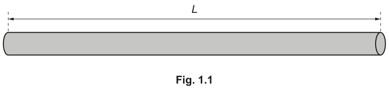
Fig. 1.1 shows a thin cylindrical metal rod of length .
One end of the rod is hit with a hammer. A stationary sound wave is set up within the rod. The rod vibrates at its resonant frequency .
A microphone placed at the other end of the rod detects the sound wave emitted from the rod. The frequency of the detected sound is also .
A number of rods of different length are available.
It is suggested that is related to by the relationship
where is the density of the metal, and and are constants.
Plan a laboratory experiment to test the relationship between and .
Draw a diagram showing the arrangement of your equipment.
Explain how the results could be used to determine values for and .
In your plan you should include:
- the procedure to be followed
- the measurements to be taken
- the control of variables
- the analysis of the data
- any safety precautions to be taken.
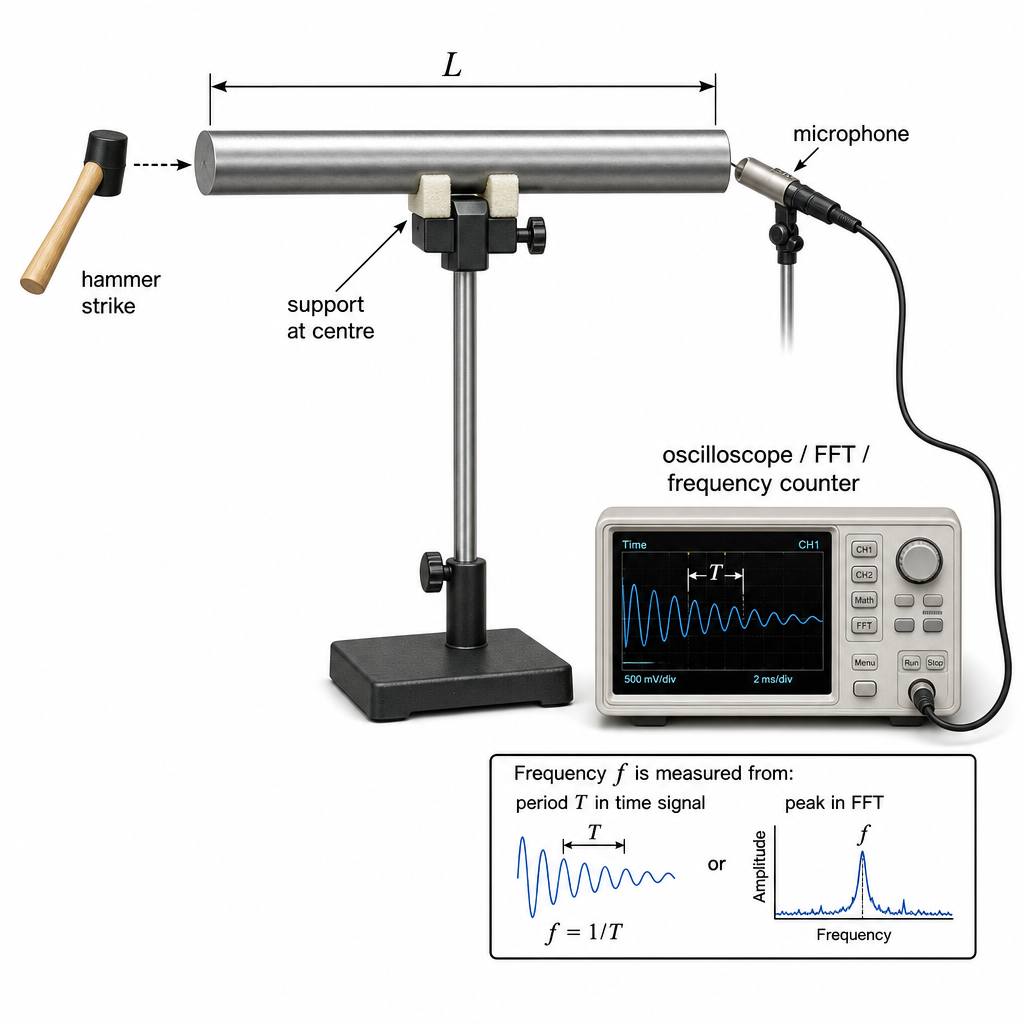
Procedure / measurements
- Choose rods of the same metal and (as far as possible) the same diameter so that and are constant; vary only .
- Measure of each rod using a metre rule/vernier calipers (same method each time).
- Support the rod at its centre (light clamp/soft supports) so the ends are free.
- Strike one end with a small hammer in the same way each time.
- Place a microphone close to the other end and connect to an oscilloscope / data-logger / frequency counter.
- Record the resonant frequency from the microphone signal (e.g. from oscilloscope time-base or FFT peak).
- Repeat strikes (e.g. 3 times) for each rod and take the mean .
Control of variables
- Same material (constant and ) and similar diameter (to avoid changing modes/damping).
- Same support position (centre), same microphone position, and similar striking method.
- Keep temperature as constant as possible.
Determination of
Measure for the metal (or use a data-book value):
- Measure mass on a balance.
- Measure diameter with a micrometer and use .
- Compute volume and then .
Analysis to determine and
Given
Take base-10 logs:
- Calculate and for each rod.
- Plot (y-axis) against (x-axis).
- Gradient .
- Intercept .
Hence
so
Safety
- Wear eye protection; ensure the rod is securely supported so it cannot fly out.
- Keep fingers away from impact point; use a small hammer and controlled ضرب.
- Consider ear protection / keep sound level moderate.
See working
Background Concept
A metal rod can support longitudinal stationary (standing) waves. At resonance, the rod vibrates strongly at a particular frequency determined by its length and the wave speed in the rod. The wave speed in a solid (for longitudinal waves) depends on material properties, and is commonly related to Young modulus and density by a relationship of the form
The question gives the suggested relationship
where and are constants for the situation. To test such a model experimentally, you vary and measure , while keeping all other relevant factors constant.
A key idea in Paper 5 is: when a relationship involves a power of a variable (here ), it is usually best tested by taking logarithms to turn it into a straight-line form.
Understanding the Question
You have several rods with different lengths . You excite a resonance by striking one end, and a microphone at the other end measures the frequency emitted.
You must:
- give a practical method to measure reliably for each ,
- identify what variables must be controlled so that changes in are due only to changes in ,
- explain a graph/data method that allows you to find both unknown constants and .
Because appears together with in the expression, you also need a value of (either measured or taken from reliable reference data).
Approach
- Choose variables: is the independent variable; is the dependent variable.
- Collect data: for each rod length, excite resonance and measure using an electronic method (oscilloscope/FFT/frequency counter). Repeat to obtain a mean.
- Control variables: ensure the rods are the same material and similar geometry; keep the measurement arrangement and conditions the same.
- Linearise: take logs of the given equation to get a straight-line graph of vs .
- Extract constants: gradient gives ; intercept gives (after using ).
Step-by-Step Reasoning
1) Data collection (getting )
- When the rod is struck, the microphone produces a voltage signal that oscillates at the sound frequency.
- An oscilloscope can measure the period from the trace, then .
- Alternatively, many data loggers/oscilloscopes can display an FFT spectrum, where the resonance shows as a peak; the peak frequency is .
- Repeating the strike reduces random variation (different strike strengths and background noise), so you average several values of .
2) Controlling variables
To test the relationship between and , you should keep constant anything else that could affect the resonant frequency:
- Material: and depend on the material, so all rods should be the same metal.
- Cross-sectional area/diameter: large changes can affect damping and which modes are most easily excited/detected; keeping diameter similar makes the comparison fair.
- Support condition: boundary conditions affect resonant frequencies. Supporting each rod in the same way (e.g. at its centre) keeps the mode pattern comparable.
- Microphone position: keeping the microphone distance/orientation fixed keeps signal strength comparable.
- Temperature: material properties (especially ) can change slightly with temperature; keep room conditions steady.
3) Determining
Since the final goal is , you need .
- If the metal is known, you may use a data-book value.
- A good experimental approach is to measure:
- mass with a balance,
- diameter with a micrometer (best for small diameters),
- compute cross-sectional area ,
- volume ,
- density .
Measuring on one representative rod is often sufficient if all rods are from the same stock.
4) Linearising to find and
Start with the given model:
Take logs (base 10, but natural logs would work similarly):
Use log laws: , , and :
Rearrange into form with and :
So, plotting (y) against (x):
- the gradient so ,
- the intercept .
Then solve for :
This uses the straight-line graph to determine both constants from experimental data.
Key Takeaways
- In a planning question, clearly state independent, dependent, and controlled variables.
- Use appropriate sensors (microphone + oscilloscope/FFT) for reliable frequency measurement.
- For relationships involving powers, use a log-log plot: gradient gives the power, intercept gives the constant.
- If a constant includes material properties (here and ), explain how will be obtained.
Common Mistakes
- Not controlling the material: using different metals would change and , invalidating the test.
- Measuring frequency vaguely (“listen for pitch”) rather than using an instrument (oscilloscope/FFT/counter).
- Plotting against directly; this will not give a straight line if .
- Forgetting to explain how to obtain from the intercept (many stop at finding ).
- Giving generic safety (“be careful”) instead of specific hazards: hammer impact, rod slipping, loud sound.
Things to Be Careful About
- Ensure the log graph is correctly defined: axes must be vs (not vs , etc.).
- Keep significant figures consistent in calculated log values and in the final constants.
- Check units conceptually: should come out in pascals ().
- Resonance detection: the largest peak may include overtones; use a consistent criterion (e.g. dominant peak) and repeat readings.
- Rod support: clamping too tightly can damp vibrations and shift resonance; use light support at the same position each time.
A student investigates an electrical circuit.
A power supply with negligible internal resistance is connected to six resistors, each of resistance , and a resistor of resistance , as shown in Fig. 2.1.
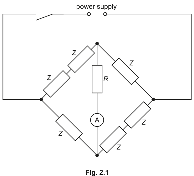
The current measured by the ammeter is .
The experiment is repeated for different values of .
It is suggested that and are related by the equation
where is the electromotive force (e.m.f.) of the power supply.
A graph is plotted of on the -axis against on the -axis.
Determine expressions for the gradient and -intercept.
gradient = ______
y-intercept = ______
Working
Given
Divide by :
So
Answer
gradient
-intercept
gradient = 3/E, y-intercept = 4Z/E
Background Concept
To analyse experimental data with a straight-line graph, we try to rewrite the given relationship in the form
where:
- is the gradient (slope),
- is the -intercept.
Here, the student plots on the -axis and on the -axis, so we want an expression of the form
Understanding the Question
You are told that
and the graph is against . So you must rearrange the equation to make the subject, and then read off:
- the coefficient of as the gradient,
- the constant term as the -intercept.
Approach
- Divide the whole equation by to create .
- Divide by to isolate .
- Compare with .
Step-by-Step Reasoning
Start with
Divide every term by :
Now divide by :
Comparing with where and :
- gradient ,
- intercept .
Key Takeaways
- Rearrange into using the variables on the axes.
- Gradient is the coefficient of the -variable; intercept is the constant term.
Common Mistakes
- Making the subject instead of .
- Stating gradient as (inverting incorrectly).
- Missing that the intercept contains .
Things to Be Careful About
- If later the graph uses in , the numerical gradient changes by a factor of (because ).
Values of and are given in Table 2.1.
Table 2.1
| 1.25 | ||
| 2.55 | ||
| 3.90 | ||
| 5.25 | ||
| 6.55 | ||
| 7.80 |
Calculate and record values of in Table 2.1.
Include the absolute uncertainties in .
Working
For ,
(1)
(2)
(3)
(4)
(5)
(6)
Answer
Record in Table 2.1:
1/I = (4440±100), (5410±150), (6250±200), (7140±260), (8000±320), (8700±380) A^-1
Background Concept
When a measured quantity is transformed, its uncertainty must also be transformed.
For a reciprocal:
the fractional (percentage) uncertainty stays the same in magnitude:
So the absolute uncertainty in is
Understanding the Question
The table gives in with an absolute uncertainty of each time. You must:
- Convert each into amperes.
- Calculate in .
- Calculate and record the absolute uncertainty in .
Approach
For each row:
- Compute .
- Compute fractional uncertainty .
- Multiply: .
- Round to match the precision implied by .
Step-by-Step Reasoning
Example (first row):
Fractional uncertainty:
So
You repeat the same method for every row.
Rounding: since the uncertainty is around , quoting to the nearest is sensible (e.g. ).
Key Takeaways
- For , fractional uncertainty in equals fractional uncertainty in .
- Always convert to SI units (here ) before calculating.
- Round the value to be consistent with the uncertainty.
Common Mistakes
- Forgetting to convert to , giving answers off by .
- Using (incorrect).
- Rounding to too many significant figures.
Things to Be Careful About
- Keep uncertainties as absolute uncertainties in (needed for error bars later).
- Ensure the unit in the table is , not .
Answer
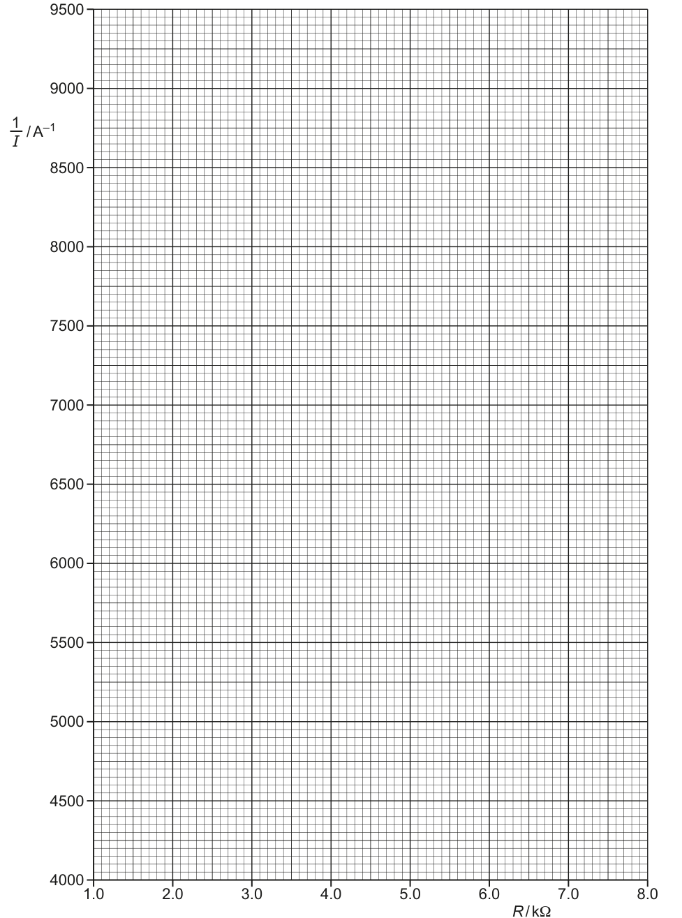
Plot the six points of from Table 2.1 on Graph 2.1.
Label axes: (x-axis) and (y-axis).
Draw vertical error bars for each point using the absolute uncertainties in .
See graph
Background Concept
A good physics graph must:
- have axes labelled with quantity and unit,
- use a sensible linear scale (usually),
- plot points accurately,
- show uncertainty using error bars.
Error bars represent the range within which the true value could lie given the measurement uncertainty. Here, only has a stated uncertainty, so only vertical error bars are required.
Understanding the Question
You have calculated and its absolute uncertainty for each . You must transfer this data onto the provided grid:
- -coordinate: in ,
- -coordinate: in ,
- vertical error bar half-length: .
Approach
- Mark each point from the table.
- For each point, draw an error bar extending up and down by the absolute uncertainty.
- Check that plotted points match the table values and lie within the axis limits.
Step-by-Step Reasoning
- Choose the given axes (already provided) and ensure your plotting is consistent.
- For example, at , if with uncertainty , the error bar should extend from to .
- Repeat for all six points.
Key Takeaways
- Error bars must be drawn using absolute (not percentage) uncertainty.
- Only draw error bars in the direction(s) where uncertainty is provided.
Common Mistakes
- Drawing horizontal error bars even though no uncertainty in is given.
- Plotting instead of .
- Omitting units on axes.
Things to Be Careful About
- Use a sharp pencil and small crosses/dots so the position is unambiguous.
- Ensure the full error bar is centred on the plotted point.
Draw the straight line of best fit and a worst acceptable straight line on your graph. Label both lines.
Answer
Draw a straight line of best fit through the plotted points.
Draw one worst acceptable straight line (steepest or shallowest) that is consistent with all the error bars.
Label the lines clearly as “best fit” and “worst acceptable”.
See graph with best-fit and worst acceptable lines
Background Concept
A best-fit line represents the overall trend of the data. When uncertainties are shown with error bars, we can estimate uncertainty in derived quantities (like gradient) by drawing a “worst acceptable” line.
A worst acceptable line is a straight line that:
- is still consistent with the data within uncertainty, meaning it passes through all (or at least is consistent with) the error bars,
- has the most extreme gradient (either steepest or shallowest) compared with the best-fit line.
Understanding the Question
You have already plotted vs with vertical error bars. Now you must:
- Draw and label the line of best fit.
- Draw and label a worst acceptable line (used later for gradient and intercept uncertainties).
Approach
- Best-fit line: balance the points so that roughly equal scatter lies above and below the line.
- Worst acceptable line: pivot the line to make the gradient as different as possible while still being consistent with the error bars.
Step-by-Step Reasoning
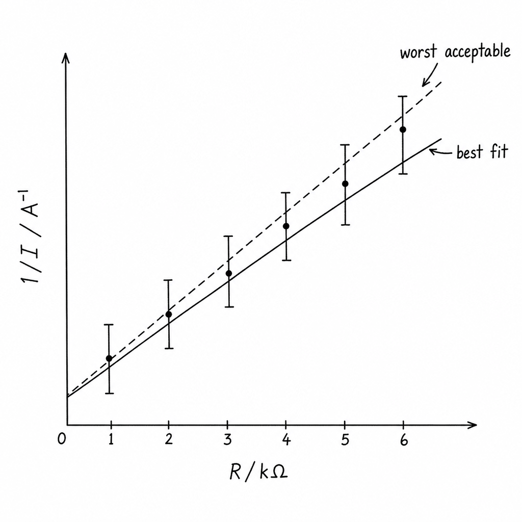
- Draw the best-fit line as a single straight line (do not join dot-to-dot).
- For the worst acceptable line, choose either:
- steepest: make the line as steep as possible while still passing within each vertical error bar, or
- shallowest: make the line as shallow as possible while still passing within each vertical error bar.
- Label both lines on the graph.
Key Takeaways
- The worst acceptable line must be justified by the error bars.
- Labelling matters: examiners need to see which line is which.
Common Mistakes
- Drawing a curve instead of a straight line.
- Drawing a worst line that ignores one or more error bars.
- Forgetting to label the lines.
Things to Be Careful About
- Use long ruler lines that extend across most of the plotted range.
- The worst line should be noticeably different from the best-fit line but still acceptable given the uncertainties.
Determine the gradient of the line of best fit. Include the absolute uncertainty in your answer.
gradient = ______
Working
Using the best-fit line (large triangle):
Using the worst acceptable line:
Absolute uncertainty:
Answer
(6.5×10^2 ± 7×10^1) A^-1 kΩ^-1
Background Concept
For a straight line graph of against , the gradient is
To reduce random reading error, you should use two points far apart on the line (a large triangle).
When error bars are present, the uncertainty in the gradient is estimated by comparing the best-fit gradient with the gradient of a worst acceptable line:
Understanding the Question
You have drawn two straight lines on your graph:
- best fit,
- worst acceptable.
You must calculate the gradient of the best-fit line and quote an absolute uncertainty using the difference between the two gradients.
Approach
- Pick two widely separated points on the best-fit line (not necessarily data points).
- Compute .
- Repeat for the worst acceptable line to get .
- Take .
Step-by-Step Reasoning
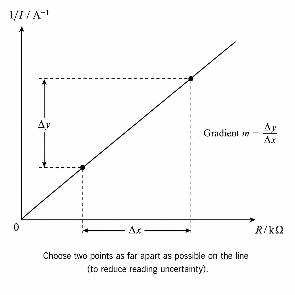
- Suppose your large triangle on the best-fit line gives approximately .
- Using two widely spaced points on the worst acceptable line gives about (a steeper line).
- Then
So you report
(Values may differ slightly depending on your drawn lines; ECF is normally applied.)
Key Takeaways
- Use a large triangle for gradient.
- Gradient uncertainty comes from best-fit vs worst acceptable line.
Common Mistakes
- Calculating gradient using two neighbouring points, giving a large percentage error.
- Using points that are not on the line (mixing in raw data points).
- Taking uncertainty as half the difference (unless the mark scheme specifically instructs it; Paper 5 typically uses the full difference).
Things to Be Careful About
- Include correct units: here .
- Read in because the axis is .
Determine the -intercept of the line of best fit. Include the absolute uncertainty in your answer.
-intercept = ______
Working
From the best-fit line, -intercept
From the worst acceptable line,
Absolute uncertainty:
Answer
(3.7×10^3 ± 3×10^2) A^-1
Background Concept
The -intercept is the value of when . For a straight line
is found by extending the line to the -axis (at ) and reading off the value.
With error bars, you can estimate uncertainty in by comparing best-fit and worst acceptable lines:
Understanding the Question
You must read the intercept from your best-fit line on the vs graph, and then find an absolute uncertainty using the worst acceptable line.
Approach
- Extend the best-fit line back to and read .
- Extend the worst acceptable line back to and read .
- Take the absolute difference as the uncertainty.
Step-by-Step Reasoning
- From the best-fit line, the intercept is about .
- From a steepest worst acceptable line, the intercept is about .
- So
Therefore
(Exact values depend on your drawn lines; ECF is normally applied.)
Key Takeaways
- The intercept is read at (extend the line if necessary).
- Intercept uncertainty comes from the spread between acceptable lines.
Common Mistakes
- Reading the intercept where the line crosses the first grid line rather than the axis.
- Using a data point as the intercept.
- Giving a percentage uncertainty when an absolute uncertainty is requested.
Things to Be Careful About
- Quote with unit .
- Use the same worst acceptable line as you used for the gradient uncertainty (consistent method).
Using your answers to (a), (c)(iii) and (c)(iv), determine the values of and . Include appropriate units.
= ______
= ______
Working
From (a):
But the graph uses , so and
Hence
Using :
And intercept :
Using and :
Answer
E = 4.6 V, Z = 4.3×10^3 Ω
Background Concept
When you plot a straight-line graph, the gradient and intercept can be used to determine constants in the original equation.
From part (a) the linear form in SI units ( in ) is:
However, if the horizontal axis uses in , then where . This multiplies the coefficient of by .
Understanding the Question
You must use your measured gradient and intercept from the graph (parts (c)(iii) and (c)(iv)) to find:
- the e.m.f. (in volts),
- the resistance (in ohms).
The key subtlety is the unit on the -axis: .
Approach
- Rewrite the straight-line equation in terms of .
- Match graph gradient and intercept to that equation.
- Solve for and , then add correct units.
Step-by-Step Reasoning
Start from
Let . Then (in ), so
So:
- gradient ,
- intercept .
Calculate :
With ,
Then calculate from :
With and ,
Key Takeaways
- Always account for axis units when linking gradient to constants.
- Use to find , then use and to find .
Common Mistakes
- Using even though the graph uses .
- Giving in without converting to when asked.
- Mixing best-fit and worst-line values for constants (unless instructed).
Things to Be Careful About
- Units: in , in .
- Consistency: use the best-fit gradient and intercept for the best estimates of and .
Working
So
Using , and , :
Answer
percentage uncertainty in
19%
Background Concept
For quantities combined by multiplication/division, fractional uncertainties add:
- If , then
- If , then
Constants such as or are exact, so they contribute no uncertainty.
Understanding the Question
You found:
- gradient with absolute uncertainty ,
- intercept with absolute uncertainty .
From these you calculated . Now you must find the percentage uncertainty in .
Approach
- Write in terms of quantities that have uncertainties (here and via ).
- Convert absolute uncertainties to fractional uncertainties.
- Add fractional uncertainties and multiply by to get percentage.
Step-by-Step Reasoning
You have
So and .
Thus
Using the representative values:
Add them:
Percentage uncertainty:
Key Takeaways
- For products/quotients, add fractional uncertainties.
- For , fractional uncertainty in equals fractional uncertainty in .
Common Mistakes
- Subtracting uncertainties for a quotient (they still add).
- Using absolute uncertainties directly without converting to fractional form.
- Forgetting to multiply by to convert to percent.
Things to Be Careful About
- Use the absolute uncertainties you obtained from best-fit vs worst acceptable lines.
- Keep consistent significant figures; percentage uncertainty is typically quoted to 1–2 significant figures.
The experiment is repeated. Determine the resistance that gives a value of of .
= ______
Working
Use
so
With , and :
Answer
9.7×10^3 Ω
Background Concept
Once you have determined constants ( and ), you can use the model equation to predict values for new conditions.
Here the relationship is linear in :
If and are constant for the power supply and the resistors, changing changes the current .
Understanding the Question
You are asked: if the current is set (or measured) to be , what value of would produce that current (using the same circuit and constants)?
Given/previously found:
- ,
- from the graph,
- from the graph.
Unknown:
- in ohms.
Approach
- Convert to amperes.
- Rearrange the equation to make the subject.
- Substitute values and calculate.
Step-by-Step Reasoning
Convert current:
Rearrange:
Substitute (using best estimates):
- ,
- ,
- .
Compute first:
Then
So is about (depending on the rounded and you use).
Key Takeaways
- Always convert mA to A before substitution.
- Rearranging first avoids algebra mistakes during substitution.
Common Mistakes
- Using instead of .
- Forgetting the factor in .
- Giving the answer in when the question asks for .
Things to Be Careful About
- Unit consistency: in volts, in amperes, and in ohms.
- Rounding: use a sensible number of significant figures consistent with and .