Physics 9702/51 — October/November 2023
Cambridge A-Level · Planning, Analysis and Evaluation · worked solutions for every part, with the mark scheme
Topics Analysis, Conclusions and Evaluation · Planning
Two coils, C and D, are placed with their axes on a straight line, as shown in Fig. 1.1.
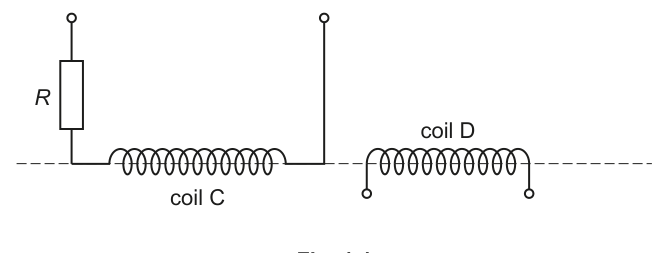
A resistor of resistance is connected in series with coil C.
A changing magnetic flux of frequency in coil C causes an electromotive force (e.m.f.) to be induced across the terminals of coil D.
It is suggested that is related to by the relationship
where is the potential difference across the resistor and coil C, and and are constants.
Plan a laboratory experiment to test the relationship between and .
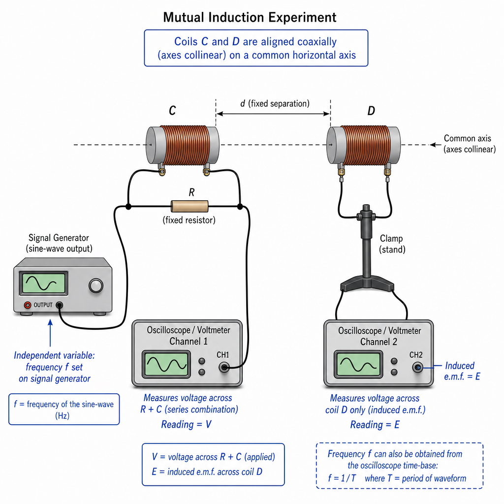
Draw a diagram showing the arrangement of your equipment.
Explain how the results could be used to determine values for and .
In your plan you should include:
- the procedure to be followed
- the measurements to be taken
- the control of variables
- the analysis of the data
- any safety precautions to be taken.
Answer
Variables
- Independent variable: frequency of the alternating current in coil C.
- Dependent variable: induced e.m.f. across coil D.
- Control variables: separation and alignment of coils, number of turns of both coils, presence/absence of any core material, resistance , and the applied p.d. amplitude across the series combination (coil C + resistor).
Apparatus (one suitable set)
- Signal generator (sine output) to drive coil C in series with fixed resistor .
- Two-channel oscilloscope (or two a.c. voltmeters) to measure and (r.m.s. or peak consistently).
- Frequency measurement from the signal generator display or oscilloscope time-base / frequency counter.
- Stands/clamps and ruler to fix and measure coil separation.
Procedure / measurements
- Mount coils C and D coaxially (axes on the same straight line) and clamp so their separation is fixed.
- Connect coil C in series with resistor to the signal generator.
- Connect a voltmeter/oscilloscope channel across the terminals of (resistor + coil C) to measure .
- Connect a high-impedance voltmeter/oscilloscope channel across coil D to measure the induced e.m.f. .
- Set a value of and adjust the signal generator output so that is kept constant (same r.m.s. or same peak for all readings).
- Record , and . Repeat the reading at least once and average.
- Repeat for a wide range of values (e.g. 6–10 values spanning at least a decade if possible) while keeping and geometry constant.
Analysis to find and
From
rearrange:
Take logs:
Plot (y-axis) against (x-axis).
- Gradient .
- Intercept , so .
Safety
- Use low voltages from the signal generator.
- Coils/resistor may heat at higher currents or frequencies: limit current, switch off between runs, and avoid touching components if warm.
- Ensure secure connections to prevent short circuits.
See working
Background Concept
A changing magnetic flux through a coil induces an e.m.f. across the coil terminals (Faraday’s law). With two coils placed close together on the same axis, an alternating current in coil C produces a changing magnetic field and hence a changing flux linking coil D. The induced e.m.f. across D depends on how fast the flux changes and how strongly the flux from C links D.
The proposed model is
where:
- is the induced e.m.f. across coil D,
- is the frequency of the changing flux (set by the driving a.c. frequency in coil C),
- is the applied potential difference across the series combination (resistor + coil C),
- is the series resistance,
- and are constants to be determined experimentally.
To test such a relationship you must:
- vary systematically,
- measure reliably,
- keep other factors constant (especially geometry and the drive amplitude, represented here by and fixed ),
- use a graph that turns the relationship into a straight line so and can be extracted from gradient/intercept.
Understanding the Question
You are asked to plan an experiment (not do a calculation). The key tasks are:
- build a setup where coil C is driven at variable frequency with a known series resistor ,
- measure the induced e.m.f. across coil D,
- measure across the supply terminals of (coil C + resistor),
- explain how your data will be analysed to find the constants and .
The statement “axes on a straight line” is an instruction to keep the coils coaxial; coupling changes strongly if the coils are moved or rotated, so the geometry must be fixed.
Approach
- Choose equipment that can provide and measure sinusoidal a.c. at variable frequency: a signal generator plus oscilloscope (ideal), or a.c. voltmeters.
- Make the only quantity you deliberately change.
- Keep constant for every run (because is predicted to be proportional to as well as dependent on ).
- For each , measure and , then compute .
- Linearise the power law by taking logs so you can plot a straight-line graph and read off and .
Step-by-Step Reasoning
1) Setting up the apparatus
You need coil C driven by an a.c. source with a fixed resistor in series (as stated). Coil D should be connected only to a measuring instrument (not a load), otherwise current in D would change the induced e.m.f. you are trying to measure.
Using an oscilloscope is particularly effective:
- It has a high input resistance, so it does not significantly load coil D.
- It can measure frequency directly from the time period, and can measure voltages as peak-to-peak (convert to peak or r.m.s. consistently).
2) Choosing variables and controls
- Independent: (set by signal generator).
- Dependent: (measured across D).
- Controls:
- Coil separation: fix with clamps and measure once with a ruler; do not move coils during the experiment.
- Alignment: keep coils coaxial and facing each other.
- : use the same resistor throughout; avoid heating that could change its resistance.
- : keep constant by adjusting the generator amplitude each time you change .
- Same waveform (sine) and same coil cores (air core/iron core) throughout.
These controls matter because mutual inductive coupling depends on geometry and magnetic properties. If the coils move or a core is introduced/removed, can change even if is unchanged.
3) Collecting data
For each frequency setting:
- Set and confirm it (generator readout or oscilloscope measurement).
- Adjust amplitude so that across (coil C + resistor) is the same as for every other reading.
- Record across coil D.
- Repeat readings (or take several cycles on the oscilloscope) and average to reduce random uncertainty.
Choose a wide frequency range and at least 6–10 readings so the log-log graph has enough points to show a clear straight-line trend.
4) Analysis to obtain and
Start from the given relationship:
Rearrange to isolate the part depending on :
This is a power law in . Taking logs gives a linear form:
So if you plot:
you expect a straight line.
- Gradient .
- Intercept .
- Hence .
(You may use instead of ; then intercept is and .)
5) Uncertainties (how to treat them well)
- Measure and with the same instrument type and consistent definition (both r.m.s. or both peak).
- Estimate uncertainties from instrument resolution (e.g. oscilloscope scale reading) and repeat measurements.
- Propagate to approximately using percentage uncertainties:
- Add error bars on the values if required; a common approximation is
Key Takeaways
- In a planning question, marks come from: a workable setup, correct variable control, valid measurements, and a clear analysis method.
- To determine constants in a power law, use a log-log plot: gradient gives the exponent, intercept gives the multiplicative constant.
- Keeping constant is essential here because depends on both and .
Common Mistakes
- Varying without keeping constant, which mixes two effects and prevents a fair test of the dependence.
- Loading coil D (e.g. connecting a low-resistance meter), causing current in D and altering the induced e.m.f.
- Changing the coil separation/alignment between readings, giving inconsistent coupling.
- Plotting vs on ordinary axes and trying to guess and without linearising.
- Mixing peak, peak-to-peak, and r.m.s. values between and .
Things to Be Careful About
- Ensure is the known fixed resistor (not the coil resistance). If heats up, its value can change; keep currents small.
- State clearly what you mean by “”: it must be the p.d. across the series combination (coil C + resistor) as defined in the question.
- Use the same coil orientation throughout; a small rotation can significantly reduce induced e.m.f.
- Use enough data points and a large enough frequency range so that the log-log graph can reliably give a gradient.
- If using an oscilloscope, set coupling and measurement mode correctly (a.c. coupling if needed; consistent voltage measurement method).
The rest of this paper
1 more questions- Q2Analysis, Conclusions and Evaluation15M