Physics 9702/51 — October/November 2022
Cambridge A-Level · Planning, Analysis and Evaluation · worked solutions for every part, with the mark scheme
Topics Analysis, Conclusions and Evaluation · Planning
A thin copper sheet is suspended from a small hole near the top of the sheet and placed in a magnetic field, as shown in Fig. 1.1.
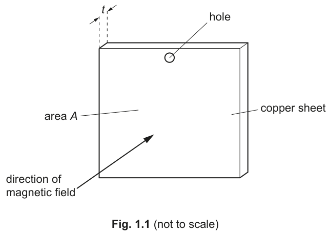
The sheet has area and thickness .
The sheet is displaced from its equilibrium position through a horizontal distance and then released so that it oscillates perpendicular to the direction of the magnetic field. The horizontal distance of the sheet from its equilibrium position is measured after five complete oscillations.
It is suggested that is related to by the relationship
where is the magnetic flux density of the field and is a constant.
Plan a laboratory experiment to test the relationship between and .
Draw a diagram showing the arrangement of your equipment.
Explain how the results could be used to determine a value for .
In your plan you should include:
- the procedure to be followed
- the measurements to be taken
- the control of variables
- the analysis of the data
- any safety precautions to be taken.
Variables
- Independent variable: area of the copper sheet.
- Dependent variable: displacement after five complete oscillations.
- Controlled variables: , , thickness , temperature, same suspension point and geometry, same number of oscillations (5), motion perpendicular to .
Apparatus and arrangement
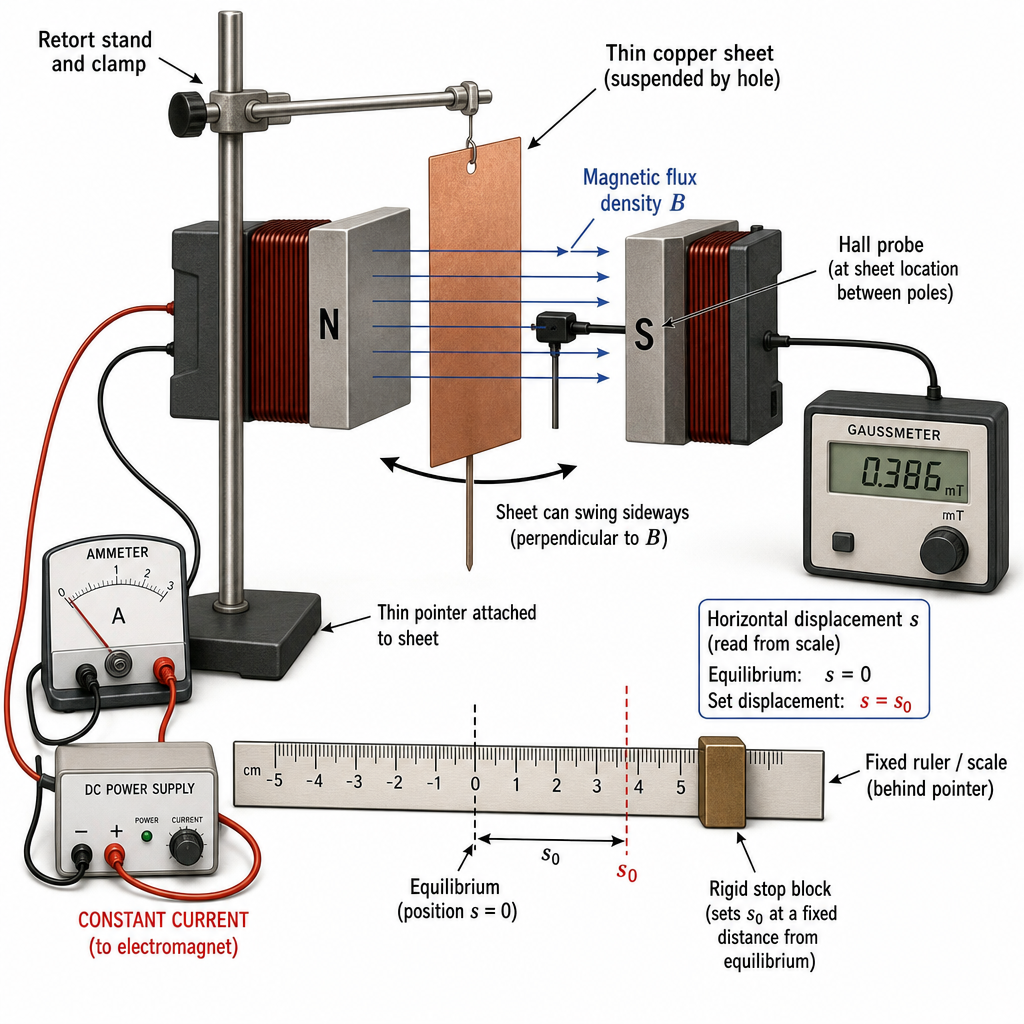
- Copper sheets (same material and thickness) with different areas .
- Electromagnet (or strong permanent magnet pair) to produce uniform .
- Gaussmeter / Hall probe to measure .
- Micrometer to measure thickness .
- Metre rule (or travelling microscope) and a fixed pointer/scale to read horizontal displacement.
- Stopwatch (to count oscillations) and a rigid stop to set the same initial displacement .
Procedure and measurements
- Choose several copper sheets of the same thickness but different areas (measure length and width to find ).
- Measure for each sheet with a micrometer and select/prepare sheets so that is the same (or use the same sheet thickness throughout).
- Set up the sheet suspended from the same hole position, centred in the magnet gap where the field is as uniform as possible.
- Measure at the position of the sheet with the Hall probe; keep magnet current constant (if using an electromagnet).
- With the sheet at equilibrium, set a pointer and scale to read horizontal displacement .
- Pull the sheet to a fixed horizontal displacement using a rigid stop/template, then release without push.
- Count five complete oscillations and then record the displacement from the scale.
- Repeat the measurement of at least three times for each and calculate a mean .
Analysis (test of relationship and determination of )
Given
Take natural logs:
For constant and , plot (y-axis) against (x-axis).
- A straight line supports the suggested relationship.
- Gradient .
Hence
Use measured values of and to calculate .
Control of variables
- Keep constant by keeping magnet current constant and checking with the probe.
- Keep constant by using sheets of the same thickness (measure with micrometer).
- Keep constant using a fixed stop and same release method.
- Keep temperature approximately constant (eddy-current damping depends on resistivity).
- Ensure sheet oscillates perpendicular to and remains within the uniform-field region.
Safety
- Keep fingers clear of magnet poles to avoid trapping.
- Secure the stand and magnet; keep strong magnets away from electronics/credit cards.
- If using an electromagnet: do not exceed current rating; beware heating of coils and leads.
- Handle copper sheet edges carefully (sharp edges).
See working
Background Concept
The motion is a damped oscillation. When a conductor moves through a magnetic field, changing magnetic flux through the conductor induces eddy currents. These currents experience magnetic forces (Lenz's law) that oppose the motion, producing a damping force.
The question suggests an exponential decay in the amplitude-like displacement after a fixed number of oscillations:
This has the general form where is constant if and are kept constant. Exponential relationships are tested most easily by taking logarithms to convert them into a straight-line graph.
Understanding the Question
You must design a practical experiment in which:
- you vary the sheet area ;
- you measure the displacement after exactly five complete oscillations (so the time interval is not fixed, but the number of cycles is);
- you keep (magnetic flux density) and the thickness constant;
- you use your results to test whether the exponential dependence on is correct;
- you then use the straight-line graph gradient (together with measured and ) to calculate the constant .
A key practical difficulty is: how do you release from the same initial displacement each time, and how do you measure consistently after five oscillations when the sheet is moving?
Approach
- Make the only deliberately-changed quantity by preparing multiple copper sheets (or cut-outs) with different areas but the same thickness.
- Use a magnet arrangement with a reasonably uniform field over the region of motion, and measure using a Hall probe so that is known (and can be checked to be constant).
- Use a fixed stop/jig so the initial displacement is reproducible.
- Measure after five oscillations using a pointer and scale (or a travelling microscope) with a consistent reference point on the sheet.
- Linearise:
so a plot of against should be a straight line with gradient , allowing to be found.
Step-by-Step Reasoning
-
Choosing and measuring
- Use several rectangular copper sheets with different length and width.
- Measure and using a ruler/vernier calipers and calculate .
- Using different sheets is usually better than cutting one sheet repeatedly, because cutting can change the suspension hole position and create bending/warping.
-
Controlling thickness
- Measure thickness using a micrometer at several points and average.
- Select sheets manufactured to the same thickness. (If varies, it would change the decay constant and spoil the test.)
-
Producing and controlling
- Place the sheet between the poles of an electromagnet or between two strong permanent magnets.
- For an electromagnet, keep the current constant using a stable power supply.
- Measure at the sheet position with a calibrated Hall probe and ensure the sheet’s motion stays within a region where is approximately uniform.
-
Setting the same initial displacement
- Put a rigid stop at a fixed horizontal distance from the equilibrium position.
- Pull the sheet gently until it just touches the stop, then release without pushing. This ensures is the same for every run.
-
Measuring after five oscillations
- Attach a thin pointer to the bottom of the sheet (or mark a reference line on the sheet) and place a scale behind it.
- Start from the moment of release and count five complete cycles (e.g. from one extreme back to the same extreme five times).
- At the instant the sheet reaches the extreme position after the 5th oscillation, read the maximum displacement from the scale.
- Repeat several times and take a mean because reading an extreme position by eye has reaction-time uncertainty.
-
Linearising and finding
Starting from
divide by and take logs:
With and controlled (constant), this is
So:
- compute for each sheet;
- plot (y) vs (x);
- the gradient gives
- Uncertainty treatment (what to do in practice)
- Estimate uncertainty in from the scale resolution and the spread in repeated readings.
- Propagate to an uncertainty in (for small uncertainties, fractional uncertainty in approximates the absolute uncertainty in ).
- Include error bars on if required and determine uncertainty in gradient using a best-fit and worst-acceptable line.
Key Takeaways
- Exponential relationships are tested by taking logarithms to obtain a straight-line graph.
- Good planning means varying one quantity (here ) while keeping others constant (, , ).
- The gradient of the linear graph is the route to extracting the constant .
- Practical marks often depend on describing how measurements are made repeatably (e.g. a stop for , repeats for ).
Common Mistakes
- Plotting against directly and expecting a straight line (it should be exponential, not linear).
- Forgetting to divide by before taking logs, or not keeping constant.
- Not measuring (you need to calculate ) or allowing to vary by moving outside the uniform field.
- Allowing thickness to change between sheets (this changes the decay factor).
- Measuring at a random time after five oscillations rather than at the extreme displacement after the 5th cycle.
Things to Be Careful About
- Ensure the oscillation is perpendicular to as stated; changing the angle changes the effective damping.
- Keep the suspension geometry the same: changing hole position changes the oscillation mode and can affect the damping.
- Use enough different areas (at least 6 values over a wide range) to make a convincing graph.
- If damping is strong, after five oscillations may be very small and hard to read; choose values so remains measurable.
- Safety with magnets (pinch hazard) and with electromagnets (heating/current limits), and sharp sheet edges.
The rest of this paper
1 more questions- Q2Analysis, Conclusions and Evaluation15M