Physics 9702/52 — May/June 2022
Cambridge A-Level · Planning, Analysis and Evaluation · worked solutions for every part, with the mark scheme
Topics Analysis, Conclusions and Evaluation · Planning
Two parallel cylindrical conductors each have a small cross-sectional area . A thin metal bar connects the two conductors, as shown in Fig. 1.1.
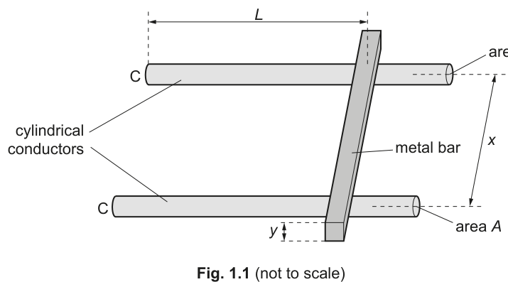
The metal bar has a square cross-section with sides of length . For each conductor, the distance between its end C and the centre of the metal bar is . The distance between the centres of the conductors is .
The ends C are connected to a power supply and the current in the conductors is measured.
It is suggested that is related to by the relationship
where is the electromotive force (e.m.f.) of the power supply, and and are constants.
Plan a laboratory experiment to test the relationship between and .
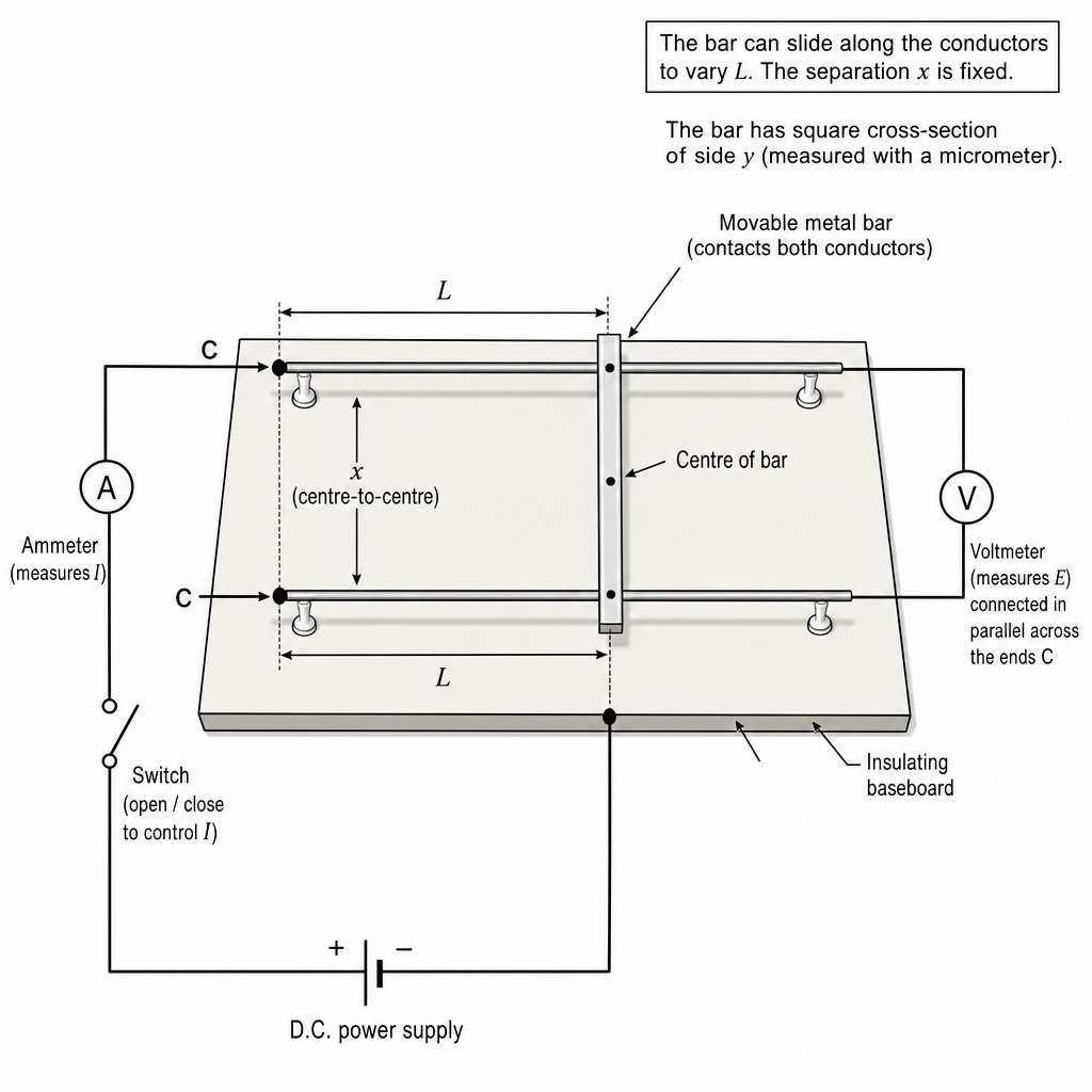
Draw a diagram showing the arrangement of your equipment.
Explain how the results could be used to determine values for and .
In your plan you should include:
- the procedure to be followed
- the measurements to be taken
- the control of variables
- the analysis of the data
- any safety precautions to be taken.
Apparatus
- Two identical cylindrical conductors mounted parallel on an insulating board
- Thin metal bar of square cross-section to bridge the conductors (fixed orientation)
- Regulated low-voltage d.c. power supply, switch
- Ammeter in series, voltmeter across ends C–C
- Metre rule / steel rule for , vernier calipers/micrometer for , micrometer for diameters
- Clamps/screw contacts/crocodile clips to ensure firm electrical contact
Procedure and measurements
- Fix the two conductors parallel so their separation is constant. Mark the end points C.
- Connect the supply to ends C with an ammeter in series and a switch. Connect a voltmeter across the ends C to measure (p.d. across the arrangement).
- Place the metal bar so it makes good electrical contact to both conductors and is perpendicular to them.
- Measure (distance from end C to the centre of the bar) using a rule. Record .
- Switch on briefly and record current and voltage . Switch off.
- Move the bar to a new position to change and repeat for at least 6–8 values of over a wide range.
- Repeat readings (or take mean of repeated and ) for each .
- Measure conductor diameter with a micrometer and calculate
Measure bar side with a micrometer. Measure conductor centre separation (e.g. measure between inner faces and add radii).
Control of variables
- Keep constant by rigidly clamping conductors.
- Use the same bar so is constant; keep its orientation the same.
- Use identical conductors so is constant.
- Minimise temperature changes (use small current, switch on only briefly, allow cooling between readings) to keep resistivity constant.
- Keep contact pressure/area constant (use screw clamps/clean contacts).
Analysis of data (to find and )
For each reading calculate .
Plot a graph of (y-axis) against (x-axis).
From
a straight line is expected with:
Safety precautions
- Use low voltage and a current-limited supply; include a switch and turn off before moving the bar.
- Avoid overheating of conductors/bar (short on-time, allow cooling); do not touch if hot.
- Secure conductors to prevent movement/short circuits.
See working
Background Concept
The suggested relationship is
The left-hand side, , has units of resistance (ohms), because . This strongly suggests the experiment is effectively measuring the total resistance between the two ends C, made up of two contributions:
- a term proportional to (resistance of the two lengths of cylindrical conductor leading to the bar), and
- a constant term for a fixed geometry ( and are constant), representing the bar/connection contribution.
A key planning idea is: if we can vary only while keeping , and constant, then should change linearly with . A straight-line graph allows us to determine constants from the gradient and intercept.
Understanding the Question
You are asked to plan an experiment (so method, measurements, control variables, analysis, and safety are what get the marks).
Given:
- Two parallel cylindrical conductors, each cross-sectional area .
- A bridging metal bar of square cross-section with side .
- Separation of the conductors is .
- For each conductor, the distance from its end C to the centre of the bar is .
- A power supply is connected to the ends C and current is measured.
Unknowns to determine: constants and .
So we must:
- change in a controlled way,
- measure and for each and calculate ,
- use a graph to obtain and .
Approach
- Choose independent and dependent variables:
- independent: (set by moving the bar position)
- dependent: (measured), and also measure so you can calculate
- Keep , , constant by using the same conductors/bar and fixing their spacing.
- Address practical limitations:
- heating changes resistivity, so limit current and take readings quickly
- contact resistance at the bar can vary, so use firm, reproducible contacts and clean metal
- Linearise: the given equation is already in straight-line form if you take and .
- Extract constants:
So measure , , to compute and .
Step-by-Step Reasoning
-
Set up the geometry
- Clamp the two conductors straight and parallel on an insulating base so is fixed.
- Ensure ends C are clearly defined (marks on the conductors help).
-
Electrical circuit
- Ammeter in series measures the current through the whole arrangement.
- Voltmeter across the ends C measures the potential difference across the conductors+bar arrangement. This is the most practical way to obtain the value used in (and avoids assuming the supply stays exactly constant under load).
-
Vary reliably
- Place the bar so it bridges the two conductors with good contact.
- Measure as the distance from end C to the centre of the bar (so you must be consistent about where you measure to).
- Move the bar to several positions to get a wide spread of values.
-
Take repeated measurements
- For each , close the switch briefly, record and , then open the switch.
- Repeat and average to reduce random variation (especially due to small contact changes).
-
Measure the fixed dimensions
- Measure conductor diameter with a micrometer and compute
- Measure bar side length with a micrometer.
- Measure carefully: for example, measure the distance between inner faces with calipers and add one diameter, or measure between outer faces and subtract one diameter. The key is that is centre-to-centre.
-
Analyse using a straight-line graph
- For each run compute .
- Plot against . If the model is correct, points should lie close to a straight line.
- Find the gradient and intercept from the best-fit line.
-
Determine and
- From
identify
(Units should be checked from these expressions; the graph gives in and in .)
Key Takeaways
- Convert the given relationship directly into a straight-line plot by choosing graph variables so it matches .
- Control variables are crucial in electrical-resistance experiments: geometry and temperature must be kept constant.
- Gradient gives one constant () and intercept gives the other (), provided you have measured , , and .
Common Mistakes
- Plotting against directly: the relationship is linear in , not necessarily in .
- Not measuring for each reading (assuming it is constant even when current changes).
- Allowing the conductors to heat up significantly, changing resistance and spoiling linearity.
- Inconsistent definition of (measuring to the bar edge sometimes and to the centre other times).
- Forgetting that is centre-to-centre separation.
Things to Be Careful About
- Contact resistance: it can dominate the intercept if the bar contact is poor; clean surfaces and use strong, repeatable clamping.
- Temperature: even modest heating changes resistivity; use low voltage/current, switch on briefly, and keep time between readings similar.
- Range and number of readings: use enough values (at least 6–8) over a wide range for a reliable gradient and intercept.
- Graph quality: use a large triangle for gradient and read intercept carefully; poor graph technique directly affects and .
- Dimensional measurements: micrometer readings for and should include appropriate precision; small errors in cause larger fractional errors in because .
The rest of this paper
1 more questions- Q2Analysis, Conclusions and Evaluation15M