Physics 9702/53 — May/June 2021
Cambridge A-Level · Planning, Analysis and Evaluation · worked solutions for every part, with the mark scheme
Topics Analysis, Conclusions and Evaluation · Planning
A student investigates the current in a coil and a resistor connected in series, as shown in Fig. 1.1.
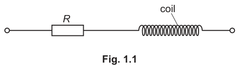
The student connects a high-voltage d.c. power supply and a switch across the series combination.
When the switch is closed, it takes time for the current in the resistor of resistance to reach a maximum value. The time is a few milliseconds.
There are a number of different unmarked resistors available.
It is suggested that the relationship between and is
where is the number of turns of wire on the coil, is the cross-sectional area of the coil, is the length of the coil and is a constant.
Design a laboratory experiment to test the relationship between and .
Explain how your results could be used to determine a value for .
You should draw a diagram, on page 3, showing the arrangement of your equipment. In your account you should pay particular attention to:
● the procedure to be followed
● the measurements to be taken
● the control of variables
● the analysis of the data
● any safety precautions to be taken.
Answer
Variables
- Independent variable: (use different unmarked resistors; measure each with a digital multimeter).
- Dependent variable: time for the current to reach its maximum steady value after the switch is closed.
- Controlled variables: same coil (fixed , , ), same power-supply setting (constant ), same shunt resistor, same switching method, keep coil temperature approximately constant.
Apparatus / arrangement
- High-voltage d.c. supply, switch.
- Coil (test inductor).
- Set of resistors.
- Small shunt resistor (low value, known) in series to measure current.
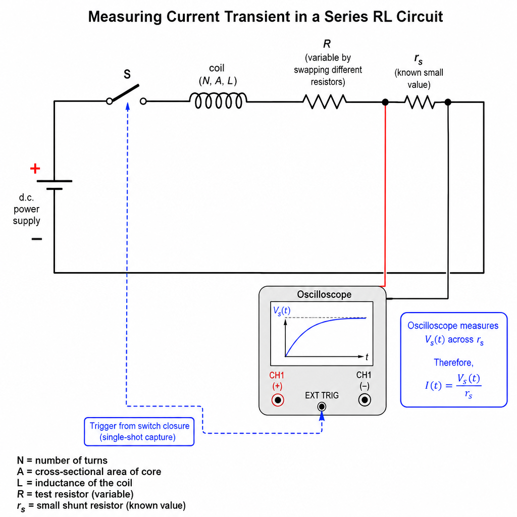
- Digital oscilloscope (or data logger) to record across .
Procedure and measurements
- Connect the series circuit: supply–switch–coil–test resistor –shunt .
- Connect the oscilloscope across so is measured; then .
- Set oscilloscope to single-shot, triggering at switch closure; choose a time-base of a few ms.
- Close the switch briefly to apply a step d.c. voltage. Record the trace of and hence .
- Determine from the plateau value. Measure from the switching instant to when the trace has reached the maximum steady value (e.g. when first becomes constant within the oscilloscope resolution, or equivalently when reaches a stated fraction such as , used consistently for all runs).
- Repeat at least 3 times for the same and take the mean . Repeat for at least 6 different values of .
Control of variables
- Use the same coil throughout (so , , constant).
- Keep constant by not changing the supply setting.
- Keep coil resistance/temperature approximately constant: keep switch closed only briefly, allow cooling time between runs, and keep current limited (choose values so coil resistance).
- Keep constant and small so it does not significantly change the chosen (or include it as a constant offset in all runs).
Analysis of data and determining
Given
Rearrange to linear form:
- Make a table of , , and mean (with uncertainties).
- Plot a graph of (y-axis) against (x-axis).
- A straight line through the origin supports the suggested relationship.
- Gradient , so
(Measure and of the coil; using calipers for radius ; from coil specification or by counting.)
Uncertainties
- Uncertainty in : from oscilloscope time-base resolution and repeat scatter; use repeats and take half-range/standard deviation.
- Uncertainty in : from multimeter resolution.
- Add error bars to the graph; uncertainty in gradient from worst acceptable line; propagate to .
Safety
- High voltage: use insulated leads, do not touch exposed conductors, switch off before changing resistors.
- Limit current (use sufficiently large and check resistor power rating to avoid overheating).
- Avoid heating the coil by keeping the switch closed only briefly.
See working
Background Concept
When a d.c. supply is suddenly connected to a series combination of a coil (inductor) and a resistor, the current does not jump instantly to its final value. The inductor produces an induced emf that opposes changes in current, so the current rises over a short time.
In a simple series circuit, the rise of current after a step in voltage is governed by an exponential approach to a steady value, with a characteristic timescale called the time constant. In general, the larger the resistance, the faster the current reaches its steady value.
The question suggests a specific relationship:
Here , , and are properties of the coil, and is a constant. If the coil is unchanged, then , , and are constant, so the equation predicts that .
Understanding the Question
You are asked to design an experiment (Paper 5 planning style) to test whether depends on in the way suggested, when a switch connects a high-voltage d.c. supply to a series coil + resistor.
So you must:
- vary (independent variable),
- measure the time for the current to reach its maximum/steady value (dependent variable),
- keep coil geometry (, , ) and other conditions constant,
- decide how to measure a current that changes over a few milliseconds,
- analyse results using a graph to check the relationship and extract .
Because the change occurs in a few ms, a meter is too slow; an oscilloscope or data logger is appropriate.
Approach
- Measure current indirectly: place a small known shunt resistor in series and measure the voltage across it; since , the measured voltage is proportional to current.
- Use single-shot recording: trigger the oscilloscope at switch closure to capture the transient.
- Repeat for multiple values and average to reduce random error.
- Linearise the given relationship: since , plot against .
- Use gradient to find because the gradient contains multiplied/divided by known coil parameters.
Step-by-Step Reasoning
1) Choosing variables
- You can control easily by swapping resistors.
- The coil parameters , , must remain fixed: therefore use the same coil for all runs.
- The time is what you are trying to see change, so it is the dependent variable.
2) Capturing a millisecond transient
A standard ammeter typically cannot resolve the current change over a few milliseconds. Instead:
- Put a small resistor in series.
- Measure across with an oscilloscope.
- Convert to current using:
This method has two big advantages:
- the oscilloscope has ms (or better) time resolution,
- measuring a voltage is easy and fast.
3) Defining and measuring
The question states “time for the current in the resistor to reach a maximum value”. In reality, the current approaches a steady value; it does not usually become perfectly constant instantly.
So you must adopt an operational definition of “reaches maximum” and keep it consistent, for example:
- measure the time from switch closure to the point where the trace first becomes flat within the oscilloscope resolution, or
- measure time to reach a stated fraction (e.g. ).
Either is acceptable in a plan as long as you state what you will do and apply it consistently.
4) Controlling variables (what could accidentally change)
- Supply voltage: keep the power supply setting fixed.
- Coil temperature: repeated large currents can heat the coil and change its resistance and inductive behaviour. Minimise by using short switching times and cooling intervals, and/or choose values that limit current.
- Extra resistances (leads, shunt, coil resistance): keep the same shunt and wiring each time. If necessary, choose values much larger than coil resistance so the tested dominates.
5) Analysis to test the relationship
Start with the given model:
Treat as constant (because the coil is unchanged). Then:
This is of the form with and .
So:
- make a table of , , and measured mean ,
- plot vs ,
- check for a straight line passing through (0,0) within uncertainties.
6) Finding from the gradient
If the graph is straight, its gradient is:
So:
You then need values for , and :
- measured with a ruler (coil length),
- from using radius measured with calipers,
- from specification or counting turns.
7) Uncertainties (what you would write to gain evaluation marks)
- Repeat traces for each to estimate random uncertainty in .
- Read using oscilloscope cursors; uncertainty is related to time-base resolution and how clearly the plateau is defined.
- Measure with a multimeter; record its uncertainty from meter resolution.
- Use error bars on (and possibly on ), draw a best-fit line and a worst acceptable line to estimate uncertainty in gradient, then propagate to .
8) Safety
High-voltage d.c. supplies can be dangerous. Sensible precautions:
- power off before changing resistors or wiring,
- use insulated leads and a properly rated switch,
- limit current to prevent overheating of resistors/coil (check power ratings),
- keep switch closed only briefly to avoid excessive heating.
Key Takeaways
- In a planning question, marks come from: clear variables, workable measurement method, control of variables, correct linearising graph, and extracting constants from gradient/intercept.
- For fast transients, use an oscilloscope and a shunt resistor to measure current indirectly.
- To test , plot against and use the gradient to find .
Common Mistakes
- Trying to measure ms-scale changes with an ammeter (too slow).
- Not stating how is defined/measured from the trace (needs a clear criterion).
- Plotting against instead of (won’t be linear for this model).
- Forgetting to measure the actual resistor values (unmarked resistors cannot be assumed correct).
- Failing to mention control of coil temperature/current (heating changes behaviour).
Things to Be Careful About
- Keep the definition of “maximum current reached” consistent across all runs.
- Ensure the shunt resistor is small and of suitable power rating; otherwise it alters the circuit significantly or overheats.
- Choose a suitable range of so that values spread out enough to see a trend (not all clustered within timing resolution).
- When extracting gradient, use a large triangle and correct units: in and in .
- When calculating , use in metres if you want SI consistency, and quote with appropriate significant figures based on measurement precision.
The rest of this paper
1 more questions- Q2Analysis, Conclusions and Evaluation15M