Physics 9702/51 — May/June 2020
Cambridge A-Level · Planning, Analysis and Evaluation · worked solutions for every part, with the mark scheme
Topics Analysis, Conclusions and Evaluation · Planning
A student investigates springs made of metal wire, as shown in Fig. 1.1.
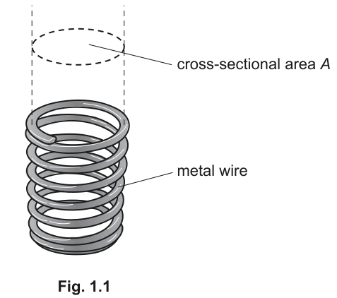
The student constructs several springs from wire of thickness . Each spring has a different cross-sectional area .
The student investigates how the spring constant varies with .
It is suggested that the relationship between and is
where is the density of the metal, is the number of turns of wire on the spring and is a constant.
Design a laboratory experiment to test the relationship between and .
Explain how your results could be used to determine a value for .
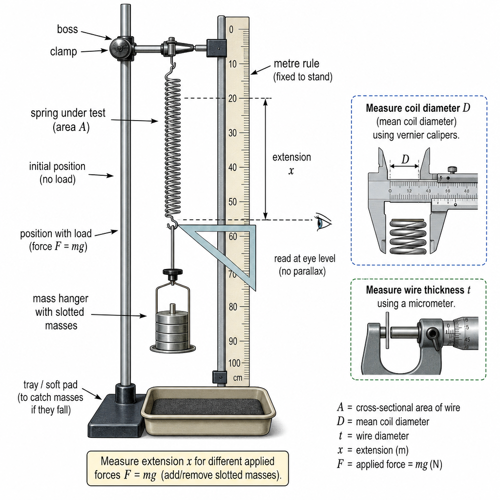
You should draw a diagram, on page 3, showing the arrangement of your equipment.
In your account you should pay particular attention to:
● the procedure to be followed
● the measurements to be taken
● the control of variables
● the analysis of the data
● any safety precautions to be taken.
Diagram
Variables
- Independent variable: spring cross-sectional area .
- Dependent variable: spring constant .
- Control variables: wire material (same ), wire thickness , number of turns (and keep the coils close-wound / similar pitch), temperature.
Apparatus
Clamp stand, boss and clamp, set of springs made from the same wire, mass hanger and slotted masses, metre rule (or mm scale) + set square / pointer, micrometer screw gauge, vernier calipers.
Procedure and measurements
- For each spring, count the number of turns .
- Measure wire thickness with a micrometer at several positions and take the mean.
- Measure the mean coil diameter using vernier calipers (several readings, mean). Calculate
- Suspend the spring vertically from the clamp. Place a metre rule beside it; use a set square/pointer to read the position of the lower end.
- Add masses in steps, ensuring the spring remains within the limit of proportionality. For each load, record extension (change in length). Take readings for loading and unloading and average.
- For each mass , calculate force .
- Plot a graph of against for each spring; the gradient gives since
Analysis to test the relationship
Given
rearrange to
For each spring calculate , then plot (y-axis) against (x-axis). A straight line through the origin supports the relationship.
Determination of
From the straight-line graph, gradient
Hence
( is taken from data for the metal used, or measured separately by mass/volume.)
Safety
- Clamp stand weighted / stable; keep feet clear of falling masses.
- Add masses gently; use safety glasses in case the spring fails.
- Do not overload the spring (avoid plastic deformation / snapping).
See working
Background Concept
A spring obeys Hooke’s law provided it is used within its limit of proportionality:
where is the applied force, is the extension, and is the spring constant (stiffness). For a given spring, a graph of against should be a straight line through the origin; its gradient is .
This planning question also tests how to test a suggested model by changing one variable (here ) while controlling others (), and then using a suitable graph to check whether the predicted dependence holds and to determine an unknown constant ().
The suggested model is
So if are constant, the prediction is a power law:
Understanding the Question
You are given several springs made from wire of the same thickness , but each spring has a different cross-sectional area (the area enclosed by the coil when viewed end-on, as in the figure). You must:
- describe a realistic laboratory method to measure for each spring,
- describe how to measure for each spring,
- ensure the other variables in the formula () are controlled/known,
- choose an analysis that tests whether varies as , and
- explain how to obtain from your results.
Because it asks you to “draw a diagram … showing the arrangement”, an apparatus set-up sketch is required.
Approach
- Make (or use) springs from the same wire material so is constant.
- Keep wire thickness the same (verify with micrometer) and keep number of turns the same (count turns).
- Vary only the coil size, so the spring’s cross-sectional area changes.
- For each spring, measure by taking several readings and finding the gradient of an – graph.
- Linearise the given relationship by rewriting it in the straight-line form
Then a plot of against should be a straight line through the origin, and the gradient gives , from which follows.
Step-by-Step Reasoning
-
Set up to measure extension accurately
- Hang the spring from a clamp stand.
- Place a metre rule vertically next to the spring.
- Use a horizontal set square or a pointer attached to the lower end of the spring so you read the scale without parallax.
-
Measure the geometry that gives
- The cross-sectional area of the spring coil can be found from its mean diameter :
- Measure using vernier calipers. Take several readings in different orientations and average (springs may not be perfectly circular).
-
Measure and control and
- Use a micrometer to measure wire thickness at several points along the wire and average. This both checks that is the same for all springs and gives a good value for later calculation of .
- Count the turns to find . If the relationship is to be tested fairly, either make all springs with identical or record and include it in the analysis (but controlling it is simpler and stronger).
-
Determine for each spring
- Add known masses in steps. For each mass, the applied force is
- Measure the extension from the change in the spring length relative to the unloaded length.
- Repeat readings (or do loading and unloading) and average to reduce random error and reduce the effect of hysteresis.
- Plot vs . The gradient is
Using a graph is better than using a single because it averages over many points and makes it easier to see if Hooke’s law holds (straight line through origin).
- Test the relationship and find
- With constant, the model predicts
- For each spring compute .
- Plot (y-axis) against (x-axis).
- If the points lie on a straight line through the origin (within uncertainties), the relationship is supported.
- The gradient satisfies
- So compute
Here can be taken from a data book for the metal. If you want to measure it, measure mass with a balance and volume by measuring length of wire used and its cross-sectional area (from ) to get density.
- Uncertainty handling (good practice for full credit)
- Uncertainty in is typically dominated by scale reading/parallax; reduce with pointer/set square.
- Uncertainty in comes from the gradient uncertainty on the – graph.
- Uncertainty in comes from uncertainty in ; since , the percentage uncertainty in is about twice that in .
- Taking multiple springs (at least 5–6 different values) improves the reliability of the straight-line test.
Key Takeaways
- Measure from the gradient of an – graph (Hooke’s law).
- Convert a coil diameter measurement into cross-sectional area using .
- Control variables that appear in the model () so only changes.
- Linearise the model by plotting against ; gradient gives a constant from which is found.
Common Mistakes
- Using a single reading of instead of a graph, losing reliability and making it hard to check Hooke’s law.
- Not stating how is measured (must relate it to a measurable diameter).
- Forgetting to control or measure and even though they appear in the formula.
- Overloading the spring so it plastically deforms; then – is not linear and is not well-defined.
- Plotting the wrong linear graph (e.g. vs rather than vs , or not explaining how comes from the gradient).
Things to Be Careful About
- Definition of : it is the area enclosed by the coil (based on the mean coil diameter), not the cross-sectional area of the wire.
- Mean diameter: for a spring, measure the coil diameter carefully; if you measure outer diameter, you may need to subtract one wire thickness to approximate mean diameter.
- Units: use SI (e.g. in m so in ; then has units ).
- Straight line through origin: the model predicts proportionality; a significant intercept suggests systematic error (e.g. zero error in extension).
- Safe working: secure clamp stand, add masses gently, keep clear of falling masses, and stay within elastic limit.
The rest of this paper
1 more questions- Q2Analysis, Conclusions and Evaluation15M