Physics 9702/53 — May/June 2019
Cambridge A-Level · Planning, Analysis and Evaluation · worked solutions for every part, with the mark scheme
Topics Analysis, Conclusions and Evaluation · Planning
A student is investigating the bending of a loaded wooden strip. Fig. 1.1 shows a rectangular strip of width and thickness overhanging the edge of a bench. A length of the strip is unsupported.
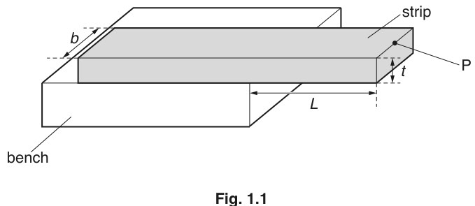
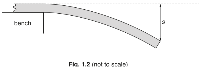
A load of mass is positioned at point P. This causes the unsupported part of the strip to bend with a deflection , as shown in Fig. 1.2.
It is suggested that the relationship between and is
where is the acceleration of free fall and is the Young modulus of the wood.
Design a laboratory experiment to test the relationship between and .
Explain how your results could be used to determine a value for .
You should draw a diagram, on page 3, showing the arrangement of your equipment. In your account you should pay particular attention to:
- the procedure to be followed
- the measurements to be taken
- the control of variables
- the analysis of the data
- any safety precautions to be taken.
Variables
- Independent variable: overhang length .
- Dependent variable: deflection at the free end (point ).
- Controls: mass/load (keep constant), same strip so and constant, position of load at the end (), same clamping position/line at bench edge, keep deflections small (within elastic limit).
Apparatus
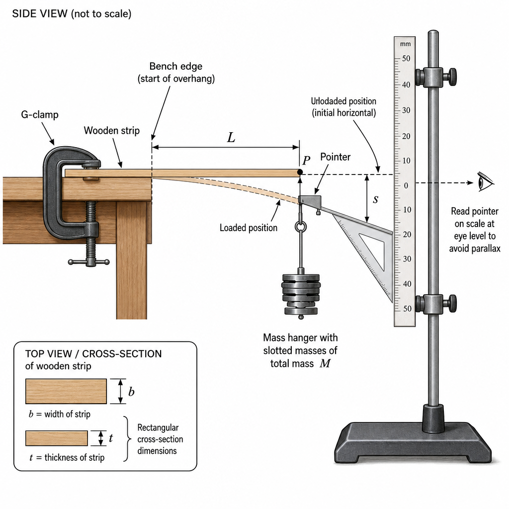
Wooden strip, bench, G-clamp, metre rule, set square, pointer/pin at end , vertical ruler (or dial gauge), mass hanger + slotted masses (total mass ), micrometer screw gauge (for ), vernier calipers (for ).
Procedure and measurements
- Clamp the strip firmly to the bench so that it overhangs; measure the unsupported length from the bench edge to point using a metre rule.
- Measure with vernier calipers and with a micrometer at several positions along the strip; take mean values.
- With no load, record the vertical position of the end against a fixed vertical scale (use a set square to reduce parallax).
- Hang a fixed load of mass at point . Allow oscillations to die away and record the new vertical position.
- Calculate deflection (loaded reading) (unloaded reading).
- Repeat step 3–5 at least twice for the same and average .
- Change by sliding the strip and re-clamping; repeat for at least 6 different values of over a suitable range.
Analysis of data (test relationship and find )
From
rearrange to
- Calculate for each reading.
- Plot a graph of (y-axis) against (x-axis).
- A straight line through the origin supports .
- Gradient is
so
Use the best-fit gradient to determine .
Control of variables (how)
- Keep the same for all readings.
- Use the same strip throughout (constant material, , ).
- Always hang the load at the same point (end of the overhang).
- Ensure clamping line is at the bench edge each time; clamp tightly to prevent slipping.
- Keep deflection small to remain in the elastic region (no permanent bend).
Safety
- Clamp securely so the strip cannot spring up or slip.
- Prevent masses falling: use a mass hanger securely; keep feet clear and do not place hands under the load.
- Keep the bench area clear to avoid tripping over hanging masses.
See working
Background Concept
A cantilever is a beam that is fixed at one end and free at the other. When a load is applied at the free end, the beam bends and the free end moves down by a deflection .
For a given material and cross-section, the stiffness depends strongly on the thickness: for a rectangular cross-section, the bending stiffness contains a factor, which is why careful measurement of is important.
The question provides a suggested relationship
where:
- is the Young modulus (a property of the material),
- is the load mass, so the force is ,
- is the overhang length (unsupported length),
- is the strip width,
- is the strip thickness.
To test how depends on , we rearrange the given equation so that the dependent variable () is on one side and the independent variable () is in a form that should give a straight-line graph.
Understanding the Question
You must plan an experiment where you:
- change deliberately,
- measure the resulting deflection caused by a fixed load at the end,
- keep other factors (, , , the material, and the loading position) constant,
- analyse the data with an appropriate graph to check the relationship,
- use the graph to calculate .
Because the relationship contains , a direct plot of against will be curved; you should instead linearise by using .
Approach
- Choose as the independent variable and vary it over a sensible range (enough to see a clear change in but not so large that the wood is permanently deformed).
- For each , measure the deflection at the same point (the free end ) with and without the load, and take the difference to reduce zero error.
- Compute and plot vs .
- Use the straight-line gradient to obtain using algebra.
Step-by-Step Reasoning
-
Set up the cantilever
- Clamp the strip to the bench so one end is fixed.
- Ensure the bench edge defines the start of the overhang; measure from this edge to the free end .
-
Choose variables and controls
- Vary only .
- Keep fixed so the applied force is constant.
- Use the same wooden strip so the material and cross-section are unchanged.
- Always apply the load at (if the load position changes, the bending moment changes and the formula would no longer apply).
-
Measure the geometry accurately
- Measure with a micrometer (better resolution than a ruler). Since the equation uses , a small error in causes a much larger percentage error in .
- Measure with vernier calipers.
- Take multiple readings along the strip and average because wood may not be perfectly uniform.
-
Measure deflection with reduced systematic error
- Put a ruler vertically near the free end and a pointer at .
- Record an initial reading with no mass.
- Hang the mass at , wait for oscillations to stop, record the new reading.
- Deflection is the difference: .
- Repeat and average to reduce random error.
-
Collect a suitable dataset
- Use at least 6 values of spread over a range.
- Avoid so large a load/overhang that the strip yields (permanent bend) because the given relationship assumes elastic behaviour.
-
Linearise and test the relationship
Starting from the given equation, rearrange to make the subject:
This has the form where should be constant if the model is correct.
- Graph and determine
- Calculate for each .
- Plot (y-axis) against (x-axis).
- If the points lie on a straight line through the origin (within uncertainty), that supports .
- Find gradient .
From the linear form,
so
- Uncertainty ideas (what you would do in practice)
- Repeat readings and use spread to estimate uncertainty.
- Uncertainty in comes from reading the metre rule and defining the bench edge and point .
- For the graph, draw a best-fit line and (if required) a worst acceptable line to estimate uncertainty in , then propagate to .
Key Takeaways
- A planning question is marked for: clear variables, workable procedure, good measurement technique, control of variables, correct linearising graph, and a clear route to the required constant ().
- Always rearrange the given relationship into a straight-line form and state what the gradient represents.
- Measure quantities that appear with powers (like ) with high precision.
Common Mistakes
- Plotting against instead of , giving a curve and no straightforward way to extract .
- Not keeping the load position fixed at the free end (changes the bending behaviour).
- Measuring from a single loaded reading without an unloaded reference (zero/parallax errors become systematic).
- Using a ruler to measure (too low precision; error in becomes large).
- Allowing the strip to slip in the clamp or exceed the elastic limit, invalidating the model.
Things to Be Careful About
- Define consistently: from the bench edge (clamp line) to the point of loading .
- Wait for oscillations of the hanging mass to stop before taking readings.
- Ensure the vertical scale is fixed and read at eye level (use a set square) to minimise parallax.
- Use consistent units (e.g. convert , , , to metres before calculating ).
- Because is cubed, take multiple micrometer readings and check for zero error on the micrometer.
The rest of this paper
1 more questions- Q2Analysis, Conclusions and Evaluation15M