Physics 9702/51 — May/June 2019
Cambridge A-Level · Planning, Analysis and Evaluation · worked solutions for every part, with the mark scheme
Topics Analysis, Conclusions and Evaluation · Planning
A student is investigating the bending of a loaded wooden strip. Fig. 1.1 shows a rectangular strip of width and thickness overhanging the edge of a bench. A length of the strip is unsupported.
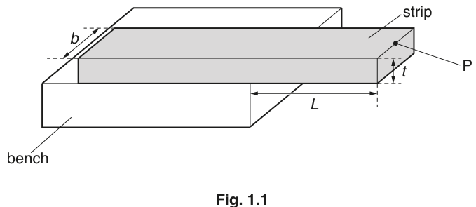
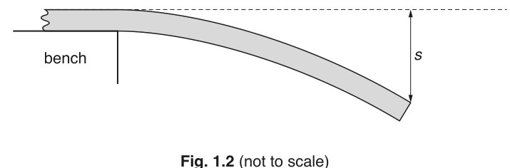
A load of mass is positioned at point P. This causes the unsupported part of the strip to bend with a deflection , as shown in Fig. 1.2.
It is suggested that the relationship between and is
where is the acceleration of free fall and is the Young modulus of the wood.
Design a laboratory experiment to test the relationship between and .
Explain how your results could be used to determine a value for .
You should draw a diagram, on page 3, showing the arrangement of your equipment. In your account you should pay particular attention to:
- the procedure to be followed
- the measurements to be taken
- the control of variables
- the analysis of the data
- any safety precautions to be taken.
Answer
Variables
- Independent variable: unsupported length .
- Dependent variable: deflection at the end (point ).
- Keep constant: load mass ; position of load at (at the free end each time); strip material; width and thickness (use same strip); orientation of strip; point of support/clamping and method of support.
Apparatus and arrangement
Wooden strip, bench with sharp edge, clamp(s)/G-clamp to prevent slipping, mass hanger + slotted masses, metre rule (for ), micrometer screw gauge/vernier callipers (for and ), dial gauge / travelling microscope / ruler with set square (for ).
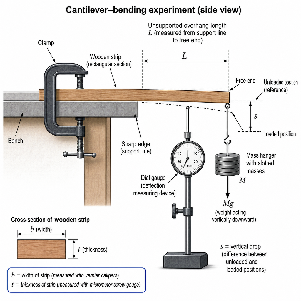
Procedure / measurements
- Clamp the strip flat on the bench so it overhangs; mark the support edge as the reference line.
- Measure and at several positions with a micrometer/vernier; take mean values.
- Set a value of by sliding the strip so the overhang from the support edge to the free end is ; measure with a metre rule.
- With no load, record the end position (zero reading).
- Hang a fixed load at point (the free end). When stationary, measure the vertical deflection (difference between loaded and unloaded readings).
- Repeat the reading of at least twice for the same and average.
- Change over a wide range (e.g. 6+ values) and repeat steps 3–6, keeping , and constant.
Analysis (test of relationship and determination of )
From
rearrange to
So plot a graph of (y-axis) against (x-axis). If the suggestion is correct, the graph is a straight line through the origin.
Gradient is
Hence
(use mean , and the best-fit gradient).
Safety
- Ensure the clamp and strip are secure so the mass cannot fall.
- Keep feet clear of the falling zone; do not overload the strip (avoid snapping / sudden release).
See working (plan and analysis).
Background Concept
A cantilever is a beam fixed at one end and free at the other. When a load is applied at the free end, the beam bends and the end drops by a vertical deflection . For small deflections (elastic behaviour), the deflection is related to the load and the geometry of the beam.
The question gives the suggested relationship
where:
- is Young modulus (a material property)
- is the load mass, so the force is
- is the unsupported length (overhang)
- is width and is thickness of the strip
- is the deflection at the free end
To test the relationship between and , we want to see whether varies as a power of (here, proportional to when other quantities are fixed). To determine , we use the gradient of a suitable straight-line graph.
Understanding the Question
You must design an experiment (Paper 5 planning style):
- Choose what you vary and what you measure.
- Explain how you will measure , , , , and keep constant.
- Explain how you will process data to check the suggested dependence of on .
- Explain how to obtain a numerical value of from your results.
- Include a labelled diagram of the apparatus and safety points.
The key idea is that you can control , , by keeping the same strip and same load, and vary only . Then measure for each .
Approach
- Choose variables: vary (independent), measure (dependent).
- Control variables: keep constant; keep the strip the same (so constant); always place the load at the same point (the free end).
- Measurement strategy:
- Measure from the support edge to the free end.
- Measure as the change in vertical position of the free end when loaded compared with unloaded to reduce zero-offset issues.
- Measure and carefully (especially because it is cubed).
- Linearise the relationship so that a straight-line graph can be used:
- Rearrange to where .
- Plot against ; gradient gives , then solve for .
Step-by-Step Reasoning
1) Setting up the cantilever
Clamp the strip to the bench so one end is fixed and a length overhangs. The support must not slip during loading; otherwise the effective changes and ruins the data.
2) Measuring and
- Use vernier callipers for .
- Use a micrometer screw gauge for .
- Take readings at several points along the strip and average because wood thickness may vary.
This matters because is in , so a small percentage error in produces roughly three times that percentage error in .
3) Measuring
For each trial:
- Slide the strip so the overhang from the support edge to the free end is the chosen .
- Measure with a metre rule; read at eye level to reduce parallax.
4) Measuring reliably
Directly measuring a small deflection with a ruler can be difficult. Better options:
- Dial gauge with its tip under the free end.
- Travelling microscope viewing a pointer attached at the free end.
- A ruler fixed vertically with a set square or pointer to align with the end.
Crucially, record an unloaded reading and a loaded reading, then
This removes systematic offsets (e.g. the strip not being perfectly horizontal initially).
Repeat readings for each and average to reduce random uncertainty.
5) Choosing the data range
Use at least 6 values of spanning as wide a range as possible while staying in the elastic region (no permanent bend). A wide range gives a clearer trend and a more reliable gradient.
6) Linearising and extracting
Start from the given expression and rearrange for :
Let
Then
with
So:
- Plot on the y-axis against on the x-axis.
- Draw a best-fit straight line.
- Determine the gradient using a large triangle.
Finally, rearrange for :
(Use consistent SI units: and in , and in , in .)
7) Considering uncertainty (what you would discuss in evaluation)
- The main uncertainty often comes from measuring and from .
- If you draw a worst acceptable line as well as the best-fit line, you can estimate uncertainty in gradient and hence uncertainty in .
Key Takeaways
- A planning question must clearly specify variables, apparatus, measurements, and how the data will be analysed.
- Testing is best done by plotting against for a straight-line check.
- Once linearised, the gradient links directly to .
- Control of variables (fixed , same strip, load always at the free end) is essential for a valid test.
Common Mistakes
- Varying as well as : then changes in cannot be attributed solely to .
- Not stating how is measured (or not using the change from unloaded to loaded).
- Plotting against instead of , which will not produce a straight line.
- Forgetting to measure and (or using a ruler for ), giving very large uncertainty in .
- Not keeping the load position fixed: moving the load changes the bending moment.
Things to Be Careful About
- Keep units consistent; use metres for all lengths when calculating .
- Ensure the strip does not slip in the clamp; any slip changes .
- Avoid large deflections: the formula assumes small deflection and elastic behaviour.
- Measure carefully; because of , even a small reading error strongly affects .
- When finding gradient, use a large triangle and compute (not ).
The rest of this paper
1 more questions- Q2Analysis, Conclusions and Evaluation15M