Biology 9700/35 — October/November 2025
Cambridge AS Level · Advanced Practical Skills · worked solutions for every part, with the mark scheme
Topics Presentation of Data and Observations · Analysis, Conclusions and Evaluation · Manipulation, Measurement and Observation · Use of the Light Microscope
Dialysis tubing is a partially permeable membrane. Some molecules such as glucose molecules can diffuse through pores in the membrane.
You are required to investigate the diffusion of glucose through the pores in dialysis tubing using two different concentrations of glucose.
You are provided with the materials shown in Table 1.1.
Table 1.1
| labelled | contents | hazard | volume / |
|---|---|---|---|
| R | 20.0% glucose solution | low | 20 |
| S | 10.0% glucose solution | low | 20 |
| G | 1.0% glucose solution | low | 30 |
| W | distilled water | low | 100 |
| Benedict's | Benedict's solution | harmful irritant | 20 |
| D1 | length of dialysis tubing in distilled water | low | — |
| D2 | length of dialysis tubing in distilled water | low | — |
If any solution comes into contact with your skin, wash off immediately with cold water. It is recommended that you wear suitable eye protection.
You will need to:
- put two different concentrations of glucose solution into dialysis tubing surrounded by water
- take a sample of the water surrounding the dialysis tubing
- test the sample for the presence of glucose.
Carry out step 1 to step 10.
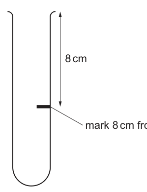
step 1 Draw a mark from the top of a large test-tube, as shown in Fig. 1.1.
step 2 Remove the dialysis tubing from beaker D1. Tie a knot in the dialysis tubing as close as possible to one end, so that the end is sealed.
step 3 The whole length of the dialysis tubing needs to be separated to allow the tubing to be filled with solution. To do this, rub the whole length of the dialysis tubing gently between your finger and thumb.
step 4 Put of 20.0% glucose solution, R, into the open end of the dialysis tubing.
step 5 Rinse the outside of the dialysis tubing by dipping it in the water in beaker D1.
step 6 Put the dialysis tubing containing R into the large test-tube and keep it in position using an elastic band as shown in Fig. 1.2.
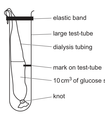
step 7 Put distilled water into the large test-tube so that the top of the water is above the level of the glucose solution in the dialysis tubing.
step 8 Start timing and leave the dialysis tubing in the distilled water for 15 minutes.
step 9 Repeat step 1 to step 7 using the dialysis tubing in the container labelled D2 and the 10.0% glucose solution, S, instead of R.
step 10 Start timing and leave the dialysis tubing in the distilled water for 15 minutes.
While you are waiting, continue with preparing the glucose standards.
Preparing glucose standards
You will need to carry out a serial dilution of the 1.0% glucose solution, G, to reduce the concentration by half between each successive dilution.
You will need to prepare four concentrations of glucose solution in addition to the 1.0% glucose solution, G.
After the serial dilution is completed, you will need to have of each concentration available to use.
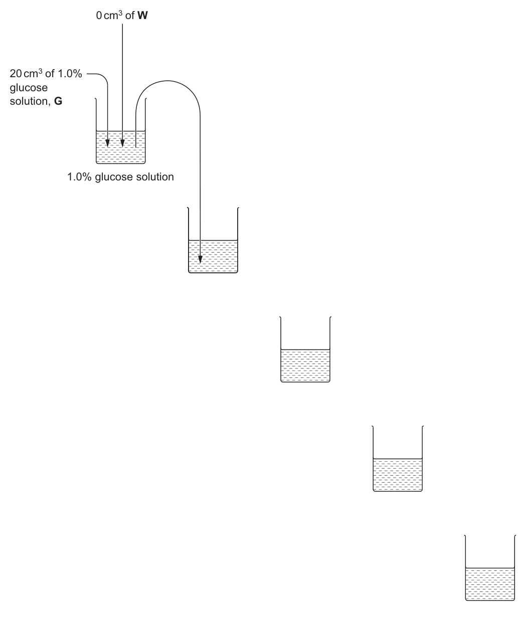
Complete Fig. 1.3 to show how you will prepare your serial dilution.
Each beaker should have:
- a labelled arrow to show the volume of glucose solution transferred
- a labelled arrow to show the volume of distilled water, W, added
- a label under the beaker to show the concentration of glucose solution.
Answer
See diagram: 0.5%, 0.25%, 0.125%, 0.0625% with 10 cm³ transfer and 10 cm³ water additions.
Background Concept
A serial dilution is a step-wise reduction in concentration by a fixed factor at each stage. For a 1:1 (halving) serial dilution, each solution in the series contains half the concentration of the previous one. The cleanest procedure is to transfer a fixed volume of the previous solution into the next beaker and top up with the same volume of diluent (water), so the final volume in each beaker stays constant while the solute is halved. This technique is widely used to produce a set of calibration standards of known concentration.
Understanding the Question
Fig. 1.3 already shows Beaker 1 containing 20 cm³ of 1.0% glucose solution (G) with 0 cm³ of water added. The candidate must complete Beakers 2–5 so that the glucose concentration halves at each step, giving four further concentrations in addition to the 1.0% starting solution. At the end of the dilution, 10 cm³ of each concentration must be available for use in the Benedict's tests.
Approach
Halve 1.0% four times: 1.0% → 0.5% → 0.25% → 0.125% → 0.0625%. Because each beaker must hold the same final volume (20 cm³), the most reliable way to halve the concentration is to transfer 10 cm³ of the previous beaker into the next and add 10 cm³ of distilled water (W).
Step-by-Step Reasoning
- Beaker 1: 1.0% (already drawn — 20 cm³ of 1.0% glucose, 0 cm³ of W).
- Beaker 2: 0.5%. Transfer 10 cm³ from Beaker 1 into Beaker 2, then add 10 cm³ of W. The 10 cm³ of 1.0% in 20 cm³ total = 0.5%.
- Beaker 3: 0.25%. Transfer 10 cm³ from Beaker 2 into Beaker 3, then add 10 cm³ of W. The 10 cm³ of 0.5% in 20 cm³ total = 0.25%.
- Beaker 4: 0.125%. Transfer 10 cm³ from Beaker 3 into Beaker 4, then add 10 cm³ of W. The 10 cm³ of 0.25% in 20 cm³ total = 0.125%.
- Beaker 5: 0.0625%. Transfer 10 cm³ from Beaker 4 into Beaker 5, then add 10 cm³ of W. The 10 cm³ of 0.125% in 20 cm³ total = 0.0625%.
Each new beaker must therefore show:
- a transfer arrow labelled '10 cm³' from the previous beaker
- a water arrow labelled '10 cm³ of W'
- a label beneath the beaker giving the new concentration (with % sign)
Key Takeaways
- A halving serial dilution produces 1.0%, 0.5%, 0.25%, 0.125%, 0.0625%.
- Equal transfer volume and diluent volume (10 cm³ each) keeps the total volume at 20 cm³ while halving the concentration.
- The % sign must appear at least once on the completed diagram (in practice it should appear on all five beaker labels).
Common Mistakes
- Forgetting the % sign on any concentration label — the mark scheme requires % at least once.
- Adding 10 cm³ of water to the 20 cm³ already present in the beaker instead of transferring 10 cm³ first — this would not halve the concentration.
- Transferring a volume other than 10 cm³, which gives the wrong concentration.
- Drawing the transfer arrow in the wrong direction (e.g. from the new beaker back into the previous one).
Things to Be Careful About
- Both the volume transferred AND the volume of water added must be clearly labelled on every new beaker.
- Each new beaker needs its own pair of arrows.
- Keep the diagonal arrangement of the printed figure — the transfer arrows curve down from one beaker to the next.
Carry out step 11 to step 19.
step 11 Set up a boiling water-bath ready for step 16.
step 12 Prepare the concentrations of glucose solutions as shown in Fig. 1.3.
step 13 Label 5 test-tubes with the concentrations prepared in step 12.
step 14 Put of each glucose concentration into the appropriately labelled test-tube.
step 15 Put of Benedict's into each of the test-tubes. Shake gently to mix.
step 16 Put the test-tube containing 1.0% glucose solution into the boiling water-bath. Start timing.
step 17 Record in (a)(ii) the time to the first colour change.
If there is no colour change after 120 seconds, stop timing and record the time as 'more than 120'.
step 18 Remove the test-tube from the boiling water-bath.
step 19 Repeat step 16 to step 18 with the other glucose concentrations.
You will need the boiling water-bath again in step 25.
Record your results in an appropriate table.
Answer
| percentage concentration of glucose (%) | time / s |
|---|---|
| 1.0 | 25 |
| 0.5 | 35 |
| 0.25 | 50 |
| 0.125 | 75 |
| 0.0625 | 110 |
Times are representative — the candidate records their own measured times. The trend must be: shorter time at higher concentration.
See table
Background Concept
The Benedict's test detects reducing sugars such as glucose. When heated with Benedict's solution, glucose reduces the blue copper(II) ions to a brick-red precipitate of copper(I) oxide. The colour sequence is blue → green → yellow → orange → brick-red. The time taken for the first colour change is inversely related to the concentration of glucose: a higher concentration reacts faster because more reducing sugar is available to react with the copper ions in a given time.
Understanding the Question
The candidate has prepared five glucose standards (1.0%, 0.5%, 0.25%, 0.125%, 0.0625%) by serial dilution. They perform a Benedict's test on each (1 cm³ of glucose + 1 cm³ of Benedict's, heated in a boiling water-bath) and record the time to the first colour change in a results table. If no colour change occurs within 120 s, the time is recorded as 'more than 120'.
Approach
Construct a table with two columns: the independent variable (glucose concentration) and the dependent variable (time to first colour change). The headings must include the unit (in the heading itself, not in the body of the table), and the independent variable heading must come before the dependent variable heading. Record whole-second times. Note the trend: higher concentration → shorter time.
Step-by-Step Reasoning
- Independent variable column heading: 'percentage concentration of glucose (%)'. The unit % is in the heading.
- Dependent variable column heading: 'time / s'. The unit s is in the heading.
- Body of the table contains only numbers — no units are repeated in each cell.
- Times are recorded to the nearest whole second (e.g. 25, 35, 50, 75, 110 — values are illustrative).
- The trend must show that the highest concentration (1.0%) gives the shortest time, and the lowest concentration (0.0625%) gives the longest time (or 'more than 120').
Key Takeaways
- Headings must have a quantity AND a unit, with the independent variable heading first.
- No units in the body of the table.
- The expected trend: shorter time = higher glucose concentration.
- Times are whole seconds.
Common Mistakes
- Putting units in the body of the table (e.g. '25 s' in each cell) — the mark scheme rejects this.
- Reversing the columns (dependent variable before independent variable).
- Forgetting the unit in the heading.
- Recording 'more than 120' for the highest concentration — the trend must be that higher concentration → shorter time.
Things to Be Careful About
- Use only whole numbers for the times.
- Write the concentrations in the same order as prepared (1.0%, 0.5%, 0.25%, 0.125%, 0.0625%) for clarity.
- Note that the Benedict's test endpoint is the FIRST colour change — not necessarily the full brick-red precipitate.
Carry out step 20 to step 23.
step 20 Label a small test-tube R1.
step 21 After 15 minutes (step 8), put a syringe into the water surrounding the dialysis tubing containing R, so that the end of the syringe is level with the mark on the test-tube. Remove from the water surrounding the dialysis tubing and put this into the test-tube labelled R1.
step 22 Label a small test-tube S1.
step 23 After 15 minutes (step 10), put a syringe into the water surrounding the dialysis tubing containing S, so that the end of the syringe is level with the mark on the test-tube. Remove from the water surrounding the dialysis tubing and put this into the test-tube labelled S1.
You will determine the concentrations of glucose in R1 and S1 by:
- carrying out the Benedict's test on R1 and S1
- using your results to estimate the concentration of glucose in R1 and S1.
Estimating the concentration of glucose in samples R1 and S1
Carry out step 24 to step 28.
step 24 Put of Benedict's into the test-tube labelled R1. Shake gently to mix.
step 25 Put the test-tube into the boiling water-bath. Start timing.
step 26 Record in (a)(iii) the time to the first colour change.
If there is no colour change after 120 seconds, stop timing and record the time as 'more than 120'.
step 27 Remove the test-tube from the boiling water-bath.
step 28 Repeat step 24 to step 27 with the test-tube labelled S1.
Record your results for R1 and S1.
result for R1 = ______
result for S1 = ______
Answer
result for R1 = ___ s
result for S1 = ___ s
(Student records their own measured times — e.g. R1 ≈ 30 s, S1 ≈ 60 s.)
Student-dependent — times for R1 and S1
Background Concept
A Benedict's test detects reducing sugars: the time to the first colour change is inversely related to the concentration. After 15 minutes of diffusion, the water surrounding each dialysis tubing will contain a small amount of glucose that has diffused out of the tubing. The Benedict's test on this water tells us how much glucose is present, by comparing the reaction time to the standard series in (a)(ii).
Understanding the Question
After 15 minutes of diffusion, the candidate uses a 1 cm³ syringe to take a 1 cm³ sample of the water surrounding the dialysis tubing containing R (20% glucose), and another 1 cm³ sample of the water surrounding the dialysis tubing containing S (10% glucose). These samples are labelled R1 and S1. A Benedict's test is then performed on each, and the time to the first colour change is recorded. If no change occurs within 120 s, the time is recorded as 'more than 120'.
Approach
Use the same technique as for the standards in (a)(ii): add 1 cm³ of Benedict's to 1 cm³ of sample, heat in the boiling water-bath, and time to the first colour change.
Step-by-Step Reasoning
- R1: sample from water surrounding dialysis tubing containing 20% glucose (R). A higher initial concentration inside the tubing means more glucose will diffuse out, so R1 should have a higher glucose concentration than S1 → shorter time to colour change.
- S1: sample from water surrounding dialysis tubing containing 10% glucose (S). A lower initial concentration inside the tubing means less glucose will diffuse out → longer time.
- Both times are recorded in whole seconds (or 'more than 120' if no change).
Representative values: R1 ≈ 30 s, S1 ≈ 60 s (illustrative; actual values depend on the candidate's experiment).
Key Takeaways
- The Benedict's test on R1 and S1 gives an indirect measure of how much glucose diffused out of the tubing.
- R1 is expected to have a higher glucose concentration than S1, and therefore a shorter reaction time.
- This is the experimental data that will be used to estimate the concentration in (a)(iv).
Common Mistakes
- Mixing up which sample is R1 and which is S1.
- Forgetting to start timing as soon as the tube enters the boiling water-bath.
- Not stopping at the FIRST colour change (waiting for full brick red).
- Recording the time in minutes rather than seconds.
Things to Be Careful About
- The sample must be taken from the water surrounding the tubing (NOT from inside the tubing).
- The 1 cm³ volume is critical for fair comparison with the standards.
- The first colour change can be subtle — watch carefully for the blue → green transition.
Use your results in (a)(ii) and (a)(iii) to estimate the percentage concentration of glucose in R1 and S1.
percentage concentration of glucose in R1 = ______ %
percentage concentration of glucose in S1 = ______ %
Answer
percentage concentration of glucose in R1 ≈ 0.5% (time similar to that recorded for the 0.5% standard)
percentage concentration of glucose in S1 ≈ 0.25% (time similar to that recorded for the 0.25% standard)
(Estimates depend on the candidate's own recorded times in (a)(ii) and (a)(iii).)
Student-dependent — estimate using the candidate's own standards
Background Concept
This is a simple application of using a calibration (standard) series to estimate an unknown. The standards in (a)(ii) provide a relationship between glucose concentration and Benedict's reaction time. By matching the reaction time of an unknown sample to the standard with the closest (or interpolated) time, the unknown's concentration can be estimated. This is the principle behind colorimetric assays and many biosensors.
Understanding the Question
The candidate must use the times recorded in (a)(ii) for the standards and the times recorded in (a)(iii) for R1 and S1 to estimate the percentage concentrations of glucose in the unknown samples. The marks are awarded for an estimate consistent with the candidate's own data.
Approach
Look up the time recorded for R1 in the standard series. The concentration whose standard has the closest reaction time is the estimate. Repeat for S1. (Alternatively, draw a graph of time vs concentration and read off the values for R1 and S1.)
Step-by-Step Reasoning
- From (a)(ii), the standard at 0.5% gives a time of (e.g.) 35 s. The standard at 0.25% gives (e.g.) 50 s.
- From (a)(iii), R1 gave a time of (e.g.) 30 s. This is closest to the 0.5% standard.
- S1 gave a time of (e.g.) 60 s. This is closest to the 0.25% standard.
- So R1 ≈ 0.5% and S1 ≈ 0.25%.
The exact values depend on the candidate's data.
Key Takeaways
- A standard series provides a calibration curve (or table) for estimating unknowns.
- The closer the unknown's reaction time to a particular standard, the more confident the estimate.
- Estimates are limited by the spacing of the standards (which is why (a)(vii) asks for improvements).
Common Mistakes
- Using a textbook value instead of the candidate's own data.
- Giving a value that doesn't match the trend of the standards (e.g. R1 lower than S1).
- Reporting an exact value when only an estimate is possible (e.g. R1 = 0.46% rather than ≈ 0.5%).
Things to Be Careful About
- The estimate must be consistent with the candidate's own data in (a)(ii) and (a)(iii).
- Use '≈' or 'about' to indicate an estimate.
- Do not claim more precision than the standard series supports.
Suggest a reason for the percentage concentrations of glucose estimated in R1 and S1 in (a)(iv).
Answer
R1 had a higher concentration of glucose than S1 because the dialysis tubing around R contained 20.0% glucose while that around S contained only 10.0%. The steeper concentration gradient between the inside of R and the surrounding water (20% → 0%) drove a faster rate of diffusion than the gradient between the inside of S and the surrounding water (10% → 0%), so more glucose molecules diffused into the water around R than around S.
R1 had a steeper concentration gradient (20% inside R vs 10% inside S), so glucose diffused out faster, giving R1 a higher glucose concentration than S1.
Background Concept
Diffusion is the net movement of particles from a region of higher concentration to a region of lower concentration, down a concentration gradient. Fick's law states that the rate of diffusion is proportional to the concentration gradient (and the surface area), and inversely proportional to the thickness of the membrane. A steeper gradient produces a faster rate of diffusion.
Understanding the Question
The candidate has estimated the glucose concentration in R1 (water around tubing R) and S1 (water around tubing S). R was 20% glucose inside; S was 10% glucose inside. The question asks why the two estimated concentrations differ.
Approach
Compare the two starting conditions: R had a higher internal concentration than S. Apply Fick's law: a steeper concentration gradient (R) produces a faster diffusion rate than a shallower gradient (S), so more glucose ends up in the surrounding water of R than of S in the same 15 minutes.
Step-by-Step Reasoning
- R contained 20% glucose inside the tubing; the surrounding water was initially 0% glucose. Concentration gradient = 20%.
- S contained 10% glucose inside the tubing; the surrounding water was initially 0% glucose. Concentration gradient = 10%.
- R had a steeper concentration gradient than S.
- By Fick's law, the rate of diffusion out of R was faster than out of S.
- After 15 minutes, the water surrounding R (sample R1) contained more glucose than the water surrounding S (sample S1).
Key Takeaways
- Diffusion rate is proportional to the concentration gradient.
- A higher internal concentration produces a steeper gradient and a faster rate of diffusion.
- This is the same principle that explains why oxygen diffuses faster from alveoli into deoxygenated blood than into oxygenated blood.
Common Mistakes
- Saying 'there was more glucose in R so more diffused out' without mentioning the concentration gradient — the mark scheme requires reference to the gradient.
- Confusing concentration gradient with simple concentration.
- Saying the diffusion rate was the same in both (ignoring the difference in gradients).
Things to Be Careful About
- The reason must mention BOTH the steeper gradient AND the faster diffusion rate (two marking points).
- The gradient is between the INSIDE of the tubing and the OUTSIDE water — not just the internal concentration.
Calculate the average rate at which the percentage concentration of glucose is increasing in the water surrounding the dialysis tubing containing R.
Show your working and give your answer to two significant figures.
average rate of increase of percentage concentration of glucose = ______ per minute
Working
Answer
≈ 0.033 % per minute (2 sig figs)
(Substitute the candidate's own R1 estimate from (a)(iv); using R1 ≈ 0.5% gives the answer above.)
≈ 0.033 % per minute (example using R1 ≈ 0.5%)
Background Concept
An average rate of change is the total change divided by the total time over which the change occurred. Here the change is the concentration of glucose that has appeared in the water outside the tubing, and the time is the 15 minutes of diffusion. This is a simple division, but the units and significant figures must be handled carefully.
Understanding the Question
The candidate must calculate the average rate at which the percentage concentration of glucose is increasing in the water surrounding the dialysis tubing containing R, using their own estimated concentration of R1 from (a)(iv) and the 15-minute diffusion time from step 8. The answer must be given to TWO significant figures.
Approach
Divide the concentration of R1 by 15 minutes to get % per minute. Round the result to two significant figures.
Step-by-Step Reasoning
- Average rate = (concentration of R1) / (15 min).
- Example: if R1 ≈ 0.5%, then rate = 0.5 / 15 = 0.0333...% per min.
- Two significant figures → 0.033% per min (the leading zeros are not significant; the 3s are).
- Other examples:
- If R1 ≈ 0.4%, rate = 0.4 / 15 = 0.0266... ≈ 0.027% per min.
- If R1 ≈ 0.3%, rate = 0.3 / 15 = 0.0200 ≈ 0.020% per min.
- If R1 ≈ 0.6%, rate = 0.6 / 15 = 0.0400 ≈ 0.040% per min.
- The unit must be 'per minute' (or '/ min' or 'min⁻¹') attached to the percentage.
Key Takeaways
- Average rate of change = change ÷ time.
- Two significant figures is the requirement — not two decimal places.
- The unit (% per min) must accompany the number.
Common Mistakes
- Giving the answer to too many or too few significant figures.
- Forgetting the unit (per minute).
- Using 5 min or 30 min instead of 15 min.
- Multiplying instead of dividing.
Things to Be Careful About
- 0.033 (to 2 sig figs) is correct; 0.03 is only 1 sig fig and would not earn the mark.
- The leading zero before the decimal is not significant; the 3s are.
- The unit should be written as '% per minute' or '%/min' — consistent with the question's wording.
Suggest how you could modify this investigation to obtain a more accurate estimate for the concentration of glucose in sample R1.
Answer
Prepare additional standard glucose solutions with much narrower concentration intervals around the estimated value for R1 — for example, standards at 0.4%, 0.45%, 0.5%, 0.55% and 0.6% if R1 is estimated at about 0.5%. The reaction time for R1 can then be matched against these closely-spaced standards to give a much more accurate estimate of its concentration.
Prepare standard glucose concentrations with narrower intervals, placed either side of the estimated R1 concentration.
Background Concept
A standard series provides a calibration for estimating unknowns, but the precision of the estimate is limited by the spacing between standards. Halving dilutions (1.0%, 0.5%, 0.25%, ...) give a broad range but widely spaced values. If the unknown's reaction time falls between two standards, the estimate is uncertain.
Understanding the Question
The candidate has estimated R1 to be (e.g.) 0.5%, but this estimate is based on widely spaced standards (the nearest are 0.25% and 1.0%). The question asks how to obtain a more accurate estimate of R1's concentration.
Approach
Reduce the spacing between standards around the estimated value of R1. Prepare standards both above and below the estimate so that the unknown can be matched against closely adjacent concentrations.
Step-by-Step Reasoning
- The current standards are 1.0%, 0.5%, 0.25%, 0.125%, 0.0625% — each step is a halving, which is too coarse around the estimated value.
- Identify the estimated R1 concentration from (a)(iv), e.g. ≈ 0.5%.
- Prepare new standards with much smaller concentration differences, e.g. 0.4%, 0.45%, 0.5%, 0.55%, 0.6% — a set of five standards spanning the region around the estimate.
- Each standard must be made with a precise transfer (e.g. 10 cm³ transfer + adjust water volume) so the concentrations are accurate.
- Perform the Benedict's test on R1 alongside these new, finer standards; match the reaction time of R1 to the closest new standard.
- The closer the spacing of the new standards, the more accurate the new estimate.
Key Takeaways
- The precision of an estimate from a standard series is limited by the spacing between standards.
- Narrowing the spacing around the estimated value gives a more precise estimate.
- The improvement is most valuable where the original standards are widely spaced (i.e., near the extremes of a halving dilution).
Common Mistakes
- Suggesting a vague improvement like 'repeat the experiment' or 'use better equipment' — these do not address the specific issue of calibration precision.
- Suggesting standards that are all on one side of the estimate (e.g. all higher than R1) — the mark scheme requires standards either side of the estimate.
- Not specifying the narrower intervals.
Things to Be Careful About
- The improvement must specifically target the precision of the concentration estimate.
- The improvement must mention BOTH narrower intervals AND standards on either side of the estimate (two marking points).
- It must be realistic — preparing solutions with concentration 0.43% or 0.567% is not practical; concentrations should be in simple, precise ratios or made with accurate pipettes.
A possible source of error when carrying out step 21 is shown in Table 1.2.
Complete Table 1.2 by stating the type of error as systematic or random, and the effect the error may have on the results.
Table 1.2
| source of error | systematic error or random error | effect on the results |
|---|---|---|
| the line at on the syringe used in step 21 actually measures a volume of and not |
Answer
Systematic error. No effect on the result because both R1 and S1 are sampled with the same miscalibrated syringe, so both are under-sampled by the same proportion; the relative difference between them is unchanged.
systematic; no effect on the results
Background Concept
Errors in measurement are classified as systematic (consistent bias in one direction, e.g. a miscalibrated instrument that always reads 5% low) or random (unpredictable variation around the true value, e.g. reading a meniscus slightly differently each time). The effect of a systematic error on a comparison depends on whether it affects both samples equally.
Understanding the Question
A 1 cm³ syringe in step 21 actually delivers 0.95 cm³ instead of 1 cm³ — a consistent 5% under-delivery. The candidate must identify this as systematic or random, and state its effect on the results.
Approach
A consistent error (every reading is 5% low) is systematic. The same syringe is used for both R1 and S1, so both samples are affected equally. The relative comparison between R1 and S1 is therefore unchanged.
Step-by-Step Reasoning
- The error is consistent: every time the syringe is used, it delivers 0.95 cm³ instead of 1 cm³. This is a systematic error (not random variation).
- The same syringe is used to sample the water around R (for R1) and the water around S (for S1).
- Both R1 and S1 therefore contain 5% less water from the surrounding than intended.
- The Benedict's test on each uses the same proportion of sample and reagent, so both R1 and S1 are affected by the same proportional error.
- The relative difference between R1 and S1 is preserved — the absolute concentration is wrong, but the comparison is unaffected.
- Hence: systematic error, no effect on the result of the comparison.
Key Takeaways
- A consistent bias is a systematic error; a fluctuating bias is a random error.
- If a systematic error affects two samples equally, the comparison between them is unaffected, even though the absolute values are wrong.
- This is why using the same instrument throughout an experiment is important.
Common Mistakes
- Classifying the error as random (because the candidate does not recognise the consistency).
- Saying the error affects the result, without specifying how or that the comparison is unaffected.
- Saying it would inflate the result (it would deflate the sampled volume, but the relative comparison is preserved).
Things to Be Careful About
- The mark scheme accepts 'systematic error' and 'no effect on the results' as the two required points.
- The candidate should think about whether the error affects the COMPARISON between R1 and S1, not just the absolute values.
Fruits contain a range of naturally occurring sugars that make them taste sweet. These sugars include glucose, fructose and sucrose. Scientists measured the mass of these sugars in apple and pineapple.
The results are shown in Table 1.3.
Table 1.3
| type of sugar | mass of sugar / g per 100 g fruit | |
|---|---|---|
| apple | pineapple | |
| glucose | 2.3 | 1.3 |
| fructose | 6.9 | 2.3 |
| sucrose | 1.9 | 5.2 |
Draw a bar chart of the data in Table 1.3 on the grid in Fig. 1.4.
Use a sharp pencil.

Answer
See bar chart
Background Concept
A bar chart is used to compare discrete categories of data. A grouped (or clustered) bar chart is used when two sub-categories are being compared across the same categories — here, two fruits (apple and pineapple) across three sugars. Bars should be drawn with uniform width, with a small gap between bars in the same group and a larger gap between groups. Lines should be ruled sharply and meet axes precisely.
Understanding the Question
Table 1.3 gives the mass of three sugars (glucose, fructose, sucrose) in 100 g of two fruits (apple, pineapple). The candidate must draw a grouped bar chart on the grid in Fig. 1.4 to compare these six values.
Approach
Use the x-axis for the categorical variable (sugar type) with three groups (glucose, fructose, sucrose), each containing two bars (apple, pineapple). Use the y-axis for the numerical variable (mass of sugar), with a scale that uses at least half the grid and is labelled at regular intervals. Plot the six bars precisely, ruling all lines.
Step-by-Step Reasoning
- x-axis label: 'type of sugar'. Three groups, evenly spaced: glucose, fructose, sucrose.
- Within each group, two adjacent bars: one for apple (e.g. shaded one way), one for pineapple (e.g. shaded another). Even bar width.
- y-axis label: 'mass of sugar / g per 100 g fruit'. Scale: 0 to 8, with labelled marks at 0, 2, 4, 6, 8 (i.e. every 2 cm if 1 cm = 1 g, or 2 g per 2 cm — the mark scheme specifies 2 g per 2 cm).
- Bar heights:
- Glucose: apple 2.3, pineapple 1.3
- Fructose: apple 6.9, pineapple 2.3
- Sucrose: apple 1.9, pineapple 5.2
- All bars drawn with horizontal and vertical lines joined precisely.
- Bars must be the same width, with a small gap within each group and a larger gap between groups.
Key Takeaways
- Grouped bar chart conventions: x-axis categorical, y-axis numerical, uniform bar widths, clear separation between groups.
- Scale must use at least half the grid, with even intervals.
- Lines must be ruled sharply and meet axes precisely.
- Each bar must be plotted accurately against the grid.
Common Mistakes
- Scale that does not use enough of the grid (e.g. 0 to 20 when max is 6.9).
- Uneven bar widths.
- Bars that do not align with the correct gridlines.
- Missing the y-axis units.
- Bars drawn freehand instead of with a sharp pencil and ruler.
- Confusing which bar is apple and which is pineapple.
Things to Be Careful About
- The mark scheme specifically requires: (1) axes labelled with both fruit names and sugar names AND y-axis units; (2) scale on y-axis as 2 g per 2 cm with labels every 2 cm; (3) all six bars plotted correctly; (4) lines joined precisely.
- The two bars within each group must be visually distinguishable (e.g. shaded differently, or labelled).
Calculate the percentage difference in the mass of sucrose per of pineapple compared to the mass of sucrose per of apple.
Show your working.
percentage difference in the mass of sucrose = ______
Working
Using the apple mass as the reference (pineapple compared to apple):
Alternatively, using the pineapple mass as the reference:
(So pineapple has either 174% or 64% more sucrose than apple, depending on which value is used as the reference.)
Answer
≈ 174 % (or ≈ 64 % if the pineapple value is taken as the reference)
≈ 174 % (or ≈ 64 %)
Background Concept
'Percentage difference' between two values can be calculated in two ways: (a) the difference as a percentage of the FIRST (reference) value, or (b) the difference as a percentage of the LARGER value. The mark scheme accepts both methods, so the candidate can use whichever is preferred.
Method A: (new − original) / original × 100, where 'new' is the value being compared to the original.
Method B: |A − B| / max(A, B) × 100.
Understanding the Question
Table 1.3 gives the mass of sucrose per 100 g of pineapple (5.2 g) and per 100 g of apple (1.9 g). The candidate must calculate the percentage difference in the mass of sucrose in pineapple compared to apple.
Approach
The mark scheme accepts two approaches:
- Approach 1 (apple as denominator): (5.2 − 1.9) / 1.9 × 100 = 173.7%, i.e. pineapple has ~174% more sucrose than apple.
- Approach 2 (pineapple as denominator): (5.2 − 1.9) / 5.2 × 100 = 63.5%, i.e. apple has ~64% less sucrose than pineapple (or pineapple has ~64% more sucrose than apple relative to its own value).
Step-by-Step Reasoning
- Identify the two values: sucrose in pineapple = 5.2 g per 100 g; sucrose in apple = 1.9 g per 100 g.
- Difference = 5.2 − 1.9 = 3.3 g per 100 g.
- Approach 1: percentage difference = 3.3 / 1.9 × 100 = 173.7% ≈ 174%. (Here apple is the reference, since the question says 'pineapple compared to apple'.)
- Approach 2: percentage difference = 3.3 / 5.2 × 100 = 63.5% ≈ 64%. (Here pineapple is the reference, giving the relative difference as a proportion of the larger value.)
The mark scheme accepts either answer — both earn the mark.
Key Takeaways
- Percentage difference = (difference between two values) / (reference value) × 100.
- The choice of reference value matters and gives different numerical answers.
- The mark scheme for this question accepts both interpretations.
Common Mistakes
- Dividing by the wrong reference value (e.g. using 5.2 when the question implies apple).
- Forgetting to multiply by 100.
- Using absolute difference in the numerator (the negative sign should not appear if the larger value is on top).
- Not showing working clearly.
Things to Be Careful About
- The mark scheme accepts BOTH 174% and 64% (or 173.7% and 63.5% if not rounded).
- The candidate should show their working with clear substitution.
M1 is a slide of a stained transverse section through a plant stem.
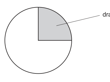
Draw a large plan diagram of the region on M1 indicated by the shaded area in Fig. 2.1.
Use a sharp pencil.
Use one ruled label line and label to identify the xylem.
Answer
A plan diagram of the shaded wedge-shaped region of M1 is drawn with the following features:
- Large size, drawn with a sharp pencil, no shading anywhere.
- A single continuous curved outline representing the epidermis at the outer edge of the wedge.
- A layer of cortex between the epidermis and the vascular tissue, drawn as a continuous band of the correct thickness.
- A continuous ring of vascular tissue crossing the wedge, with at least three vascular bundles visible.
- The vascular bundles drawn in the correct proportion relative to the cortex and the pith.
- A central region of pith (cells) inside the vascular ring.
- No individual cells drawn anywhere — only tissue boundaries as lines.
- One ruled label line, drawn with a ruler, ending exactly on the xylem within the vascular ring, labelled 'xylem'.
See plan diagram with label to xylem.
Background Concept
A plan diagram is a low-power, outline-only drawing of a specimen. It shows the arrangement and proportion of tissues — not individual cells. Conventions for plan diagrams are heavily rewarded in CIE Paper 3 marking:
- Use sharp, single, continuous lines (no sketchy/fuzzy outlines).
- Do not shade any region.
- Do not draw individual cells anywhere — only the boundaries between tissues.
- Make the drawing large (it should fill most of the space provided).
- Keep proportions accurate — the cortex should not be drawn thicker than the vascular tissue if it isn't, etc.
- Labels use a ruled line that ends precisely on the structure; no arrowheads.
A plant stem in transverse section typically shows (outside → inside): epidermis → cortex → vascular tissue (xylem on the inside, phloem on the outside) → pith. The way these tissues are arranged (continuous ring vs separate bundles, number of rings, presence/absence of pith) is what distinguishes a young dicot stem, a monocot stem, a root, etc.
Understanding the Question
The question asks the candidate to draw a plan diagram of a specific wedge-shaped region of the stem section M1 indicated in Fig. 2.1. The diagram must show the tissues correctly, follow plan-diagram conventions, and include a labelled xylem. The marks reward size, shading rules, proportions, shape of the outline and vascular tissue, and the label.
The marking scheme tells us that M1 has continuous vascular tissue (one ring, cells in the centre). This is the key feature distinguishing M1 from Fig. 2.2, which has separate vascular bundles.
Approach
The strategy is to:
- Identify the tissues in M1 — look down the microscope and decide where the epidermis, cortex, vascular tissue, and pith lie in the wedge.
- Sketch lightly first to get the proportions right.
- Trace the final outlines in sharp, single, continuous pencil lines.
- Add the one required label (xylem) using a ruler; the label line must touch the structure being labelled and the label written clearly at the end of the line.
- Check there is no shading and no cells drawn anywhere.
Step-by-Step Reasoning
- Appropriate size and no shading — fill most of the answer space; leave all interior regions blank (no stippling, hatching, or pencil shading). This single mark covers both points.
- Correct section of stem — the outline should match the curved outer boundary of the stem in the wedge, with the inner tissues drawn in proportion. The wedge should not look like a rectangle or circle.
- At least three vascular bundles, correct proportion, no cells — the vascular tissue crosses the wedge as a band; the candidate must show at least three recognisable bundle 'bulges' in that band. Critically, do not draw the individual cells of the cortex or pith — only their boundaries.
- Correct outline shape and continuous vascular tissue — the epidermis must be drawn as a single smooth curve, and the vascular tissue must be drawn as a continuous ring, not as separate islands. This matches the biology of M1 (continuous ring of vascular tissue).
- Label line to xylem — a single straight line drawn with a ruler, ending on the xylem tissue (the inner part of the vascular band), labelled 'xylem'. Do not label any other structures.
Key Takeaways
- A plan diagram is about tissue arrangement, not cellular detail.
- Conventions (sharp lines, no shading, no cells, large size, ruled label lines) are themselves worth marks — they are easy to lose and easy to earn with care.
- Recognising whether the vascular tissue forms a continuous ring or separate bundles is a key diagnostic feature of stem anatomy.
Common Mistakes
- Drawing individual cells inside tissues — this loses the 'no cells' mark and the diagram becomes a high-power drawing rather than a plan.
- Shading any region (e.g. filling in the pith with pencil). Plan diagrams must be unshaded.
- Using unruled, wobbly label lines, arrowheads, or labels that don't end on the structure.
- Drawing the vascular tissue as separate bundles when in fact it is continuous in M1 (this is the diagnostic feature being tested).
Things to Be Careful About
- The label line must end on the xylem, not on the phloem or cortex.
- The diagram should be of the shaded wedge in Fig. 2.1, not of the whole section.
- Make the vascular tissue a continuous ring (M1's biology) and show its inner edge clearly so the pith is distinct.
Observe the xylem vessel elements in the stem on M1.
Select a group of four adjacent xylem vessel elements.
Each xylem vessel element must touch at least one other xylem vessel element.
- Make a large drawing of this group of four xylem vessel elements.
- Use one ruled label line and label to identify the wall of one xylem vessel element.
Answer
A high-power drawing of four adjacent xylem vessel elements is drawn with the following features:
- Large size; sharp, continuous pencil lines; no shading.
- Only four xylem vessel elements drawn; each one touches at least one other (e.g. arranged as a 2 × 2 cluster or a row of four in contact).
- Each xylem vessel element drawn with two lines around it, representing the thick lignified wall.
- Where two elements touch, three lines are drawn (the two walls of the touching elements).
- Correct shape — the elements are roughly circular/polygonal, with a clear empty lumen.
- No contents drawn inside the lumen (xylem vessel elements are dead and empty at maturity).
- One ruled label line, drawn with a ruler, ending on the wall of one xylem vessel element, labelled 'wall'.
See drawing of four xylem vessel elements with label to wall.
Background Concept
Xylem vessel elements are dead, hollow cells with thickened, lignified walls. They are joined end-to-end and the end walls dissolve to form continuous xylem vessels for water transport. Each element therefore has a thick wall around a hollow lumen with no cytoplasm, nucleus or organelles. Under the microscope they appear as large empty polygonal or circular cells with prominent walls.
In a high-power biological drawing, the double-line convention represents the cell wall — because the cell wall itself has thickness and is built of layers. Where two cells touch, each contributes its own two lines, giving three lines in total (one line from each cell's wall plus the shared middle line representing the middle lamella / shared wall). This is one of the most heavily tested conventions in CIE Paper 3.
Understanding the Question
The candidate must select four adjacent xylem vessel elements on M1 such that each element touches at least one other. The high-power drawing must follow biological-drawing conventions: sharp lines, double walls, three lines where elements touch, empty lumens, no shading, and one label to the wall of one element.
The marks reward: (1) appropriate size and sharp continuous lines; (2) only four elements drawn, each touching at least one other; (3) two-line walls and three lines where elements touch; (4) correct shape; (5) label line to the wall.
Approach
The strategy is to:
- Move to high power on the microscope.
- Identify a region where you can clearly see four adjacent xylem vessel elements with each touching at least one other — usually where vessels are densely packed.
- Note the actual shape (round, polygonal, oval) and the relative sizes of the elements before drawing.
- Sketch the cluster lightly, then trace with sharp single lines, drawing two lines around each element.
- Where elements touch, draw three lines (one shared boundary between the two walls).
- Leave lumens empty (no dots, no nucleus, no shading).
- Add one ruled label line to the wall of one element, labelled 'wall'.
Step-by-Step Reasoning
- Appropriate size, sharp continuous lines — draw large (fill most of the space); lines must be single, crisp pencil strokes with no fuzzy gaps.
- Only four xylem vessel elements, each touching at least one other — pick exactly four. A common error is to draw five because an extra element creeps in. Arrangements that satisfy 'each touches at least one other': a row of four in contact, a 2 × 2 cluster, or a 'T' shape.
- Two lines around each, three lines where elements touch — for every element draw its outer wall as two parallel lines. Where two elements share a wall, the shared boundary is drawn as three lines (two walls pressed together).
- Correct shape — match the observed shape: roughly circular if vessels were round in T.S., polygonal if angular. Sizes should reflect relative sizes seen.
- Label line to the wall — one ruler-drawn line ending exactly on one wall (the pair of lines making up that wall), labelled 'wall'. Do not label the lumen or any other feature.
Key Takeaways
- High-power drawings of plant cells must use the double-line wall convention.
- Three lines where two cells touch is a signature mark — forgetting it costs marks.
- Xylem vessel elements are dead at maturity, so the lumen is empty in a mature section — do not draw cytoplasm, nucleus or organelles.
Common Mistakes
- Drawing only one line around each element (looks like an animal cell or a plan diagram outline).
- Drawing five or six elements instead of exactly four.
- Drawing cytoplasm, a nucleus or organelles inside the lumen.
- Labelling the lumen instead of the wall, or labelling with an arrowhead or unruled line.
- Drawing elements that don't actually touch, failing the 'each touches at least one other' rule.
Things to Be Careful About
- The two lines around each element should be parallel and close together — not so far apart that they look like a single thick wall with an internal space.
- The lumen must be truly empty (no shading, no stippling, no nucleus dot).
- Only one label is required; adding extra labels (lumen, xylem, vessel, etc.) is not wrong but is unnecessary.
Fig. 2.2 is a photomicrograph of a stained transverse section of a stem from a different plant to M1.
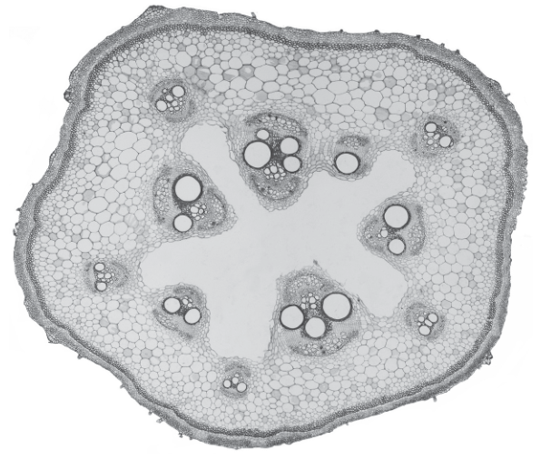
Identify three observable differences, other than colour, between the stem section on M1 and the stem section in Fig. 2.2.
Record these three observable differences in an appropriate table.
Answer
| Feature | M1 | Fig. 2.2 |
|---|---|---|
| Shape of stem outline | circular | five-sided (pentagonal) |
| Vascular bundles | one ring | two rings |
| Vascular tissue | continuous | in separate bundles |
| Central tissue (pith) | cells present | no cells (hollow centre) |
Any three of the four rows above earn the three marks for observable differences; the table with both specimen headings earns the fourth mark.
Three observable differences recorded in a table with headings for M1 and Fig. 2.2.
Background Concept
Comparing two specimens is a core Paper 3 skill. The candidate must base the comparison only on observable features seen under the microscope or in the photomicrograph — not on prior knowledge of what species they are. The comparison should be presented in a table with clear headings for each specimen so that the differences can be read at a glance.
For plant stems, the key observable features are:
- Outline shape (circular, polygonal, how many sides).
- Arrangement of vascular tissue (continuous ring vs separate bundles; one ring vs two rings).
- Presence/absence of pith (cells in the centre vs hollow centre).
- Number and size of vascular bundles.
- Position of xylem and phloem within each bundle.
Understanding the Question
The candidate is given two stem sections — the actual slide M1 viewed down the microscope and the photomicrograph Fig. 2.2 printed in the paper — and asked to identify three observable differences, other than colour, recording them in an appropriate table. The mark scheme awards one mark for the table with correct headings and three marks for three valid differences.
The marking scheme provides four possible differences (shape, vascular bundle arrangement, vascular tissue continuity, central tissue), so any three of these earn full marks.
Approach
- Look at M1 carefully under the microscope (or, where photomicrographs of M1 are provided, study them) and note its observable features.
- Examine Fig. 2.2 in the question paper and note its observable features.
- Pick three valid differences — features that are clearly observable (not requiring interpretation) and that are present in one specimen but absent or different in the other.
- Record them in a table with the specimens as column headings and the feature as the row heading.
Step-by-Step Reasoning
The valid differences, taken from the mark scheme, are:
- Shape of outline — M1 is circular; Fig. 2.2 is five-sided (pentagonal).
- Vascular bundles — M1 has one ring; Fig. 2.2 has two rings (one near the cortex, one around the hollow centre).
- Vascular tissue — M1's vascular tissue is continuous (a single connected ring); Fig. 2.2's vascular tissue is in separate, discrete bundles.
- Central tissue (pith) — M1 has cells in the centre (a pith); Fig. 2.2 has no cells in the centre (the centre is hollow).
Any three of these differences are creditable. The fourth mark is for the table format — the candidate must draw a table with headings for both M1 and Fig. 2.2 so the reader can see the comparison at a glance.
A common trap is to give a difference such as 'M1 has xylem inside, phloem outside' — this is not an observable difference between the two specimens (both have this arrangement), it is a feature common to both. The differences must be features present in one but not the other.
Another trap is to base a difference on colour — the question explicitly rules this out ('other than colour').
Key Takeaways
- Differences must be observable in the specimens shown — not inferred from prior knowledge.
- The four key observable features for stems are outline shape, vascular bundle arrangement, vascular tissue continuity and central tissue.
- A comparative table with specimen headings is the expected format and earns its own mark.
Common Mistakes
- Including colour as a difference (explicitly ruled out).
- Giving a difference that is not actually observable in both specimens (e.g. asserting a feature that cannot be seen).
- Writing differences as long sentences rather than in a structured table with headings.
- Using vague descriptions such as 'M1 has more vascular bundles' without saying what the actual arrangement is.
- Omitting the pith/no pith difference because the hollow centre is so obvious it is overlooked.
Things to Be Careful About
- The 'two rings vs one ring' point is subtle — count the rings carefully. Fig. 2.2 has bundles near the periphery and bundles near the hollow centre, so it has two rings; M1 has a single ring of continuous vascular tissue.
- Do not list a feature that is shared by both — it isn't a difference.
- The hollow centre of Fig. 2.2 is not pith — there are no cells there. State 'no cells in centre' or 'hollow centre', not 'no pith', because the mark scheme rejects vague wording.
Fig. 2.3 shows a photomicrograph of a stage micrometer scale that is being used to calibrate an eyepiece graticule.
One division, on either the stage micrometer scale or the eyepiece graticule, is the distance between two adjacent lines.
The length of one division on the stage micrometer in Fig. 2.3 is .
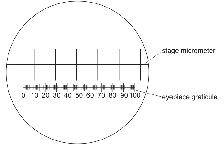
Calculate the actual length of one eyepiece graticule unit shown in Fig. 2.3.
Give your answer in micrometres (µm).
Show your working and give your answer to three significant figures.
actual length of one eyepiece graticule unit = ______
Working
From Fig. 2.3:
- 100 eyepiece graticule units span 10 stage micrometer divisions.
- 1 stage micrometer division = = .
- Therefore 100 eyepiece graticule units = .
Answer
actual length of one eyepiece graticule unit = µm
100 µm
Background Concept
An eyepiece graticule is a tiny scale (usually 100 divisions) etched into a glass disc that sits inside the microscope eyepiece. Its divisions look the same size regardless of the magnification of the objective lens — but the actual length that each division represents depends on which objective lens is in use.
A stage micrometer is a slide with a precisely known scale (each division = or typically). To calibrate the eyepiece graticule for a particular objective lens, the two scales are superimposed and aligned. The number of eyepiece graticule divisions that line up with a known length on the stage micrometer is then counted. From this:
Once calibrated, the eyepiece graticule can be used to measure any specimen on that microscope at that objective lens simply by counting divisions.
Understanding the Question
The candidate is given Fig. 2.3 showing the stage micrometer and eyepiece graticule superimposed. They are told that one division on the stage micrometer is . They must read the alignment and work out the actual length (in µm) of one eyepiece graticule division, to three significant figures.
From Fig. 2.3, 100 eyepiece graticule divisions span 10 stage micrometer divisions — the graticule's full 0 to 100 range lines up with 10 mm of stage micrometer scale. This is the alignment the markscheme requires.
Approach
- Read the number of eyepiece graticule divisions that align with one stage micrometer division (or vice versa).
- Convert the stage micrometer length to µm.
- Divide to find the actual length of one eyepiece graticule division.
- Express the answer to three significant figures (a specific marking requirement).
Step-by-Step Reasoning
- Counting the alignment — 100 eyepiece graticule units span 10 stage micrometer divisions. So one stage micrometer division (1.0 mm) = 10 eyepiece graticule units.
- Unit conversion — . Therefore 10 eyepiece graticule units = .
- Divide — 1 eyepiece graticule unit = .
- Three significant figures — write the answer as (not or etc.).
Equivalently: 100 eyepiece graticule units = = , so 1 eyepiece graticule unit = .
Key Takeaways
- An eyepiece graticule must be calibrated for each objective lens because its actual length per division changes with magnification.
- The conversion is essential in microscope work.
- Always quote answers to the number of significant figures the question asks for — here, three.
Common Mistakes
- Forgetting to convert mm to µm (writing the answer as instead of ).
- Quoting an answer to the wrong number of significant figures.
- Reading the alignment incorrectly (e.g. counting the wrong number of eyepiece divisions across one stage division).
- Forgetting to show the working — the mark scheme requires both division and unit conversion steps.
Things to Be Careful About
- The question explicitly says three significant figures — already has three significant figures, but be careful not to round a different value to fewer.
- Make sure the units in the final answer match the units requested (µm, not mm).
Fig. 2.4 is the same photomicrograph as that shown in Fig. 2.2. This was taken with the same microscope and the same lenses used to take the photomicrograph in Fig. 2.3.
The eyepiece graticule has been placed across the length of a vascular bundle.
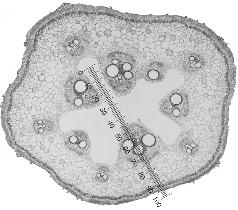
Use the calibration of the eyepiece graticule unit from (c)(i) to calculate the actual length of the vascular bundle in Fig. 2.4.
Show your working and use appropriate units.
actual length of the vascular bundle = ______
Working
From Fig. 2.4:
- The vascular bundle spans approximately 70 eyepiece graticule units (read from the graticule placed across the bundle).
- From (c)(i): 1 eyepiece graticule unit = .
Converting to a more convenient unit:
Answer
actual length of the vascular bundle = µm ( = )
7000 µm (7.0 mm)
Background Concept
Once the eyepiece graticule has been calibrated (part (c)(i)), any specimen on the same microscope with the same objective lens can be measured simply by counting graticule divisions across the feature of interest and multiplying by the calibration factor.
The relationship is:
Units must be consistent — if calibration is in µm, the result is in µm; convert to mm if a more convenient unit is wanted.
Understanding the Question
Fig. 2.4 is the same photomicrograph as Fig. 2.2, taken with the same microscope and same lenses as Fig. 2.3 (the calibration image). An eyepiece graticule has been placed across a vascular bundle. The candidate must:
- Read the number of eyepiece graticule divisions spanned by the vascular bundle.
- Multiply by the calibration from (c)(i) ( per division) to obtain the actual length.
- Show the working and use appropriate units (µm or mm).
Approach
- Identify the two ends of the vascular bundle on the graticule and read the number of divisions spanned (e.g. 70).
- Multiply by the calibration from (c)(i).
- Convert to a sensible unit (µm or mm) and present the final answer.
Step-by-Step Reasoning
- Reading the graticule — in Fig. 2.4 the graticule runs diagonally across the vascular bundle. The bundle starts at approximately graticule mark 5 and ends at approximately mark 75, so the bundle spans about 70 eyepiece graticule divisions.
- Applying the calibration — 70 divisions × = .
- Unit conversion — the question says 'use appropriate units'. is awkward; converting gives . Either is acceptable, but converting makes the size of the vascular bundle easier to interpret.
- Error carried forward (ecf) — if the candidate's calibration in (c)(i) was wrong but they correctly multiplied the graticule reading by their calibration value, full marks are still awarded here.
Key Takeaways
- The calibration is specific to the objective lens in use — change the lens and you must recalibrate.
- 'Appropriate units' means a unit that makes the size of the specimen sensible — µm for cells, mm for whole organs. Either is fine if stated correctly.
- Error carried forward allows the candidate to recover from a wrong calibration in (c)(i) provided the multiplication in (c)(ii) is performed correctly.
Common Mistakes
- Forgetting to show the working — the mark scheme explicitly requires the multiplication step to be visible.
- Reading the bundle length as the total graticule span (e.g. 100) rather than the actual span covered by the bundle.
- Mixing units — writing the calibration in mm but applying it in µm, or vice versa.
- Not converting to appropriate units (giving an answer in pm, m, or with no unit).
Things to Be Careful About
- The reading of the bundle length is the only measurement-dependent step — different candidates will read it slightly differently (e.g. 65 vs 70 vs 75 divisions). Any reasonable reading is creditable, and the working carries the mark.
- Always state the unit with the answer — bare numbers without units are not credited in CIE marking.