Biology 9700/38 — May/June 2025
Cambridge AS Level · Advanced Practical Skills · worked solutions for every part, with the mark scheme
Topics Presentation of Data and Observations · Manipulation, Measurement and Observation · Analysis, Conclusions and Evaluation · Use of the Light Microscope
Catalase is an enzyme found in yeast cells. It catalyses the breakdown of hydrogen peroxide to produce water and oxygen, as shown in Fig. 1.1.
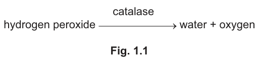
Fig. 1.1
You will investigate the effect of copper sulfate on the progress of this reaction. You will do this by stopping the reaction after 5 minutes and measuring the concentration of hydrogen peroxide remaining.
Potassium manganate(VII) is used to measure the concentration of hydrogen peroxide.
You are provided with the materials shown in Table 1.1.
Table 1.1
| labelled | contents | hazard | volume / |
|---|---|---|---|
| Y | yeast suspension | none | 20 |
| H | hydrogen peroxide solution | irritant | 20 |
| C | 1.0% copper sulfate solution | irritant | 30 |
| A | dilute sulfuric acid | irritant | 30 |
| P | potassium manganate(VII) solution | harmful | 30 |
| W | distilled water | none | 150 |
If any solution comes into contact with your skin, wash off immediately under cold water.
You should wear suitable eye protection.
It is recommended that you wear gloves when using A and P.
You will need to carry out a serial dilution of the 1.0% copper sulfate solution, C, to reduce the concentration by half between each successive dilution.
You will need to prepare four concentrations of copper sulfate solution in addition to the 1.0% copper sulfate solution, C.
After the serial dilution is completed, you need to have of each concentration available to use.
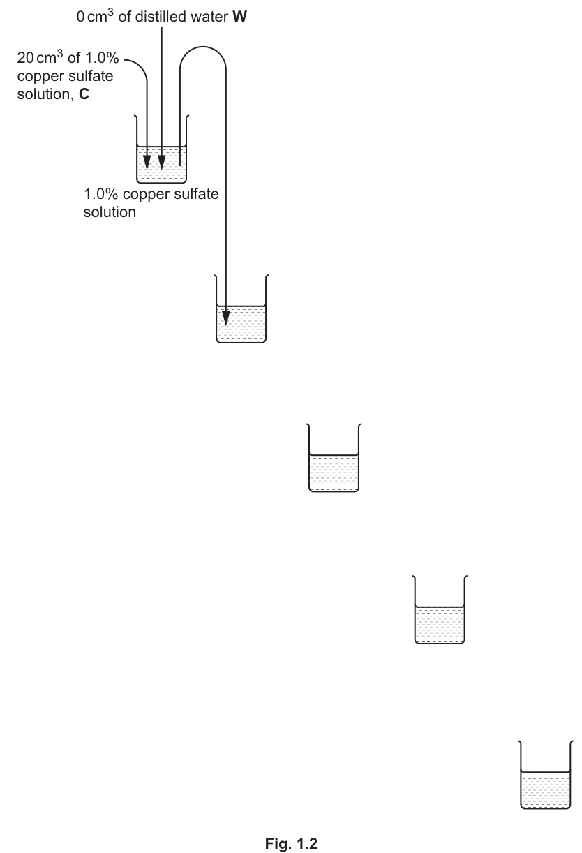
Complete Fig. 1.2 to show how you will prepare your serial dilution.
Each beaker should have:
- a labelled arrow to show the volume of copper sulfate solution transferred
- a labelled arrow to show the volume of distilled water, W, added
- a label under each beaker to show the concentration of the copper sulfate solution.
Answer
Complete Fig. 1.2 by adding the following to beakers 2 to 5:
- A curved arrow from the previous beaker labelled " of copper sulfate solution" (transferred into the new beaker)
- A vertical arrow into each beaker labelled " of distilled water W"
- A concentration label under each beaker:
- Beaker 2:
- Beaker 3:
- Beaker 4:
- Beaker 5:
Each beaker contains a total of (the transferred plus the of water added). The first beaker (already given) contains of 1.0% CuSO plus of water, also a total of . Of the in each beaker, is used in the experiment and is transferred to the next beaker (except the last, where all is used).
Serial dilution: 1.0% → 0.5% → 0.25% → 0.125% → 0.0625%, with 10 cm³ transferred and 10 cm³ of water W added at each step
Background Concept
A serial dilution is a standard laboratory technique used to prepare a range of solutions of decreasing concentration. Each successive solution is made by diluting the previous one by a fixed factor. When the dilution factor is 2 (i.e. halving the concentration each time), the volumes transferred and added must be equal: transferring of the previous solution and adding of diluent (distilled water W) gives a total of at half the original concentration. This is the simplest and most common form of serial dilution, and it gives a geometric series of concentrations (1, 1/2, 1/4, 1/8, 1/16, ...).
Understanding the Question
Fig. 1.2 shows the start of a serial dilution: the first beaker contains of 1.0% copper sulfate solution C, and the candidate is asked to extend the dilution through four more beakers so that five concentrations (1.0% plus four new ones) are available. Each beaker should contain a labelled arrow showing the volume of copper sulfate solution transferred, a labelled arrow showing the volume of distilled water W added, and a label showing the concentration under the beaker. The end result must give of each concentration available for the experiment.
Approach
To halve the concentration at each step while still leaving of usable solution in the previous beaker, transfer from the previous beaker and add of distilled water W. The new beaker will contain at half the concentration. The candidate then uses of this in the experiment and transfers to the next beaker. The concentrations halve each time: 1.0% → 0.5% → 0.25% → 0.125% → 0.0625%.
Step-by-Step Reasoning
- Beaker 1 (already given): of 1.0% CuSO + water = at 1.0%. Of this, is used in the experiment and is transferred to beaker 2.
- Beaker 2: of 1.0% CuSO + water = at . Of this, is used in the experiment and is transferred to beaker 3.
- Beaker 3: of 0.5% CuSO + water = at 0.25%. Of this, is used and is transferred to beaker 4.
- Beaker 4: of 0.25% CuSO + water = at 0.125%. Of this, is used and is transferred to beaker 5.
- Beaker 5: of 0.125% CuSO + water = at 0.0625%. All is used in the experiment (no further beaker).
The final answer for Fig. 1.2 is four beakers (2 to 5), each showing a curved arrow from the previous beaker labelled " of copper sulfate solution", a vertical arrow into the beaker labelled " of distilled water W", and a concentration label underneath (0.5%, 0.25%, 0.125%, 0.0625%).
Key Takeaways
- A serial dilution halves the concentration when equal volumes are transferred and added.
- Each beaker in this series holds , providing for use and to pass on (except the last, where all is used).
- The five concentrations are 1.0%, 0.5%, 0.25%, 0.125% and 0.0625%.
Common Mistakes
- Using unequal volumes (e.g. transferring and adding would dilute by a factor of 4, not 2).
- Labelling the wrong concentration under a beaker, or skipping a value in the sequence.
- Forgetting to include the volume labels on the arrows.
- Putting the wrong total volume in the beakers (each must end with for the procedure to work).
Things to Be Careful About
- The candidate must show transferred (not ); if all were transferred, the previous beaker would be empty.
- The candidate must add of water W to each of beakers 2 to 5 (not , which is correct only for beaker 1).
- The concentration labels must appear in the correct order along the diagonal: 0.5%, 0.25%, 0.125%, 0.0625%.
Carry out step 1 to step 7.
step 1 Prepare the concentrations of copper sulfate solution as shown in Fig. 1.2.
step 2 Label test-tubes with the concentrations prepared in step 1.
step 3 Put of the 1.0% copper sulfate solution into the appropriately labelled test-tube.
step 4 Put of each of the other concentrations of copper sulfate solution, as prepared in step 1, into the appropriately labelled test-tube.
step 5 Stir the yeast suspension, Y, and put of Y into each test-tube. Shake the test-tubes gently to mix. Wait for 2 minutes.
step 6 Put of hydrogen peroxide solution, H, into each test-tube. Shake gently to mix. Wait for 5 minutes.
step 7 After 5 minutes, put of sulfuric acid, A, into each test-tube. Shake gently to mix.
The addition of sulfuric acid stops the breakdown of hydrogen peroxide.
You will now compare the concentration of hydrogen peroxide remaining in each test-tube using potassium manganate(VII) solution, P.
- When a drop of P is added to hydrogen peroxide solution, you will see a pink colour that quickly turns colourless as P reacts with the hydrogen peroxide.
- You will continue adding P, one drop at a time, until the end-point is reached.
- The end-point is when the pink colour stays for at least 5 seconds.
- You will count the number of drops to reach the end-point.
- The greater the concentration of hydrogen peroxide, the more drops of P are needed to reach the end-point.
Carry out step 8 to step 14.
step 8 Fill the syringe labelled P with solution P.
step 9 Wipe the outside of the syringe with a paper towel.
step 10 Hold the syringe labelled P over the test-tube containing the lowest concentration of copper sulfate solution. Release one drop of P into the test-tube.
step 11 Shake the test-tube to mix. Observe the colour to see if the end-point is reached. The end-point is when the pink colour stays for at least 5 seconds.
step 12 Repeat step 10 and step 11, counting the total number of drops released until the end-point is reached. You may need to refill the syringe with P.
step 13 Record in (a)(ii) the number of drops of P added. If the end-point has not been reached with 30 drops, record the result as 'more than 30'.
step 14 Repeat step 8 to step 13 with each of the other concentrations of copper sulfate solution prepared in step 1.
Record your results in an appropriate table.
Answer
Record the results in a table with the independent variable (concentration of copper sulfate / %) to the left of the dependent variable (number of drops of P):
| Concentration of copper sulfate / % | Number of drops of P |
|---|---|
| 0.0625 | (student value) |
| 0.125 | (student value) |
| 0.25 | (student value) |
| 0.5 | (student value) |
| 1.0 | (student value) |
Representative results (illustrative):
| Concentration of copper sulfate / % | Number of drops of P |
|---|---|
| 0.0625 | 7 |
| 0.125 | 10 |
| 0.25 | 14 |
| 0.5 | 19 |
| 1.0 | 25 |
All values should be recorded as whole drops. The expected trend is that as the concentration of copper sulfate increases, the number of drops of P needed to reach the end-point also increases.
Two-column table: concentration of copper sulfate (%) vs number of drops of P, with the trend that higher CuSO4 concentrations give more drops of P (e.g. 7 → 25 as 0.0625% → 1.0%)
Background Concept
A results table should have a clear heading for each column that includes both the quantity being measured and its unit. The independent variable (the one deliberately varied by the experimenter) is placed in the left column, and the dependent variable (the one measured) in the right column. If the same procedure is repeated, replicates can be added as additional columns. Here the candidate records a single set of readings (one per concentration), so two columns are sufficient.
Understanding the Question
The candidate has carried out the procedure in step 1 to step 14 and now needs to record, in an appropriate table, the number of drops of potassium manganate(VII) P needed to reach the end-point for each of the five concentrations of copper sulfate prepared in step 1. The independent variable is the concentration of copper sulfate; the dependent variable is the number of drops of P. The mark scheme requires:
- a heading for the independent variable to the left of the dependent variable
- a heading for the dependent variable (number of drops of P)
- a value for each of the five concentrations
- whole drops only
- the expected trend (the higher the concentration of CuSO, the more drops of P)
Approach
Construct a two-column table with the concentration of copper sulfate (in %) on the left and the number of drops of P on the right. Record one whole number per row, in ascending or descending order of CuSO concentration. The expected trend reflects the inhibition: as CuSO increases, less catalase is active, less HO is broken down in the 5 minutes, and so more P is needed to react with the remaining HO.
Step-by-Step Reasoning
- Identify the independent variable: concentration of copper sulfate (%). Place in the left column with the unit.
- Identify the dependent variable: number of drops of P. Place in the right column.
- List the five concentrations: 0.0625%, 0.125%, 0.25%, 0.5%, 1.0% (or in reverse order).
- Record the number of drops of P needed to reach the end-point for each concentration. Each value is a whole number (or 'more than 30' if the end-point is not reached within 30 drops).
- Check the trend: as CuSO concentration rises, the number of drops of P should rise. If the trend is reversed, suspect a procedural error (e.g. the CuSO may have been added in the wrong order, or the same pipette may have been used between concentrations without rinsing).
Key Takeaways
- A table of results should have a clear heading for each column including the unit.
- The independent variable is on the left; the dependent variable is on the right.
- In an inhibition experiment, more inhibitor means more substrate remains, so the dependent variable (related to substrate concentration) should rise with the inhibitor.
Common Mistakes
- Omitting the unit from the column heading (e.g. just 'concentration of copper sulfate' without the %).
- Putting the dependent variable (drops of P) to the left of the independent variable (concentration of CuSO).
- Recording non-integer values (e.g. 14.5 drops) when the procedure specifies whole drops.
- Recording a trend that decreases with concentration (which would suggest the inhibitor is acting as an activator — not what the data show).
Things to Be Careful About
- Whole drops only — the procedure involves counting each drop, so fractional drops cannot be recorded.
- 'More than 30' is an acceptable entry if the end-point is not reached; the mark scheme accepts this.
- The order of rows can be ascending or descending concentration; either is acceptable as long as the trend is clear.
Describe the effect of changing the concentration of copper sulfate solution on the concentration of hydrogen peroxide remaining in the test-tubes.
Answer
The higher the concentration of copper sulfate, the higher the concentration of hydrogen peroxide remaining in the test-tube.
The higher the concentration of copper sulfate, the higher the concentration of hydrogen peroxide remaining
Background Concept
Catalase is an enzyme in yeast cells that breaks down hydrogen peroxide (HO) into water and oxygen. Copper sulfate is a known inhibitor of catalase: at higher concentrations, the active site of the enzyme is more likely to be occupied by copper ions, reducing the rate at which catalase breaks down HO. After a fixed time (5 minutes), if more HO remains, it means less breakdown has occurred, i.e. the enzyme has been more inhibited.
Understanding the Question
The candidate has measured the number of drops of P needed to reach the end-point for each CuSO concentration. Because more drops of P are needed when more HO is present, the number of drops is a direct indicator of the HO concentration remaining after 5 minutes. The question asks the candidate to describe the relationship between CuSO concentration and HO remaining.
Approach
State the trend in plain words: as CuSO increases, HO remaining also increases. The mark scheme expects a single sentence linking the two variables in the correct direction.
Step-by-Step Reasoning
- Look at the table: as CuSO increases from 0.0625% to 1.0%, the number of drops of P increases (e.g. 7 → 25 in the representative table).
- More drops of P means more HO is present, because each drop reacts with a fixed amount of HO until the end-point is reached.
- Therefore, more HO remains at higher CuSO concentrations. This reflects greater inhibition of catalase.
Key Takeaways
- A positive correlation between CuSO concentration and the number of drops of P means a positive correlation between CuSO concentration and the HO remaining.
- The biology: copper sulfate inhibits catalase, so the enzyme breaks down less HO in 5 minutes when more inhibitor is present.
Common Mistakes
- Stating the wrong direction (e.g. 'the higher the CuSO, the lower the HO remaining') — this is the opposite of what the experiment shows.
- Being vague ('CuSO affects HO') without specifying the direction.
- Confusing the cause and effect (e.g. saying 'more HO causes more CuSO' instead of the other way around).
Things to Be Careful About
- The question asks for a description, not an explanation. A single sentence stating the trend is sufficient.
- The exact phrasing matters: the mark scheme looks for 'the higher the concentration of copper sulfate, the higher the concentration of hydrogen peroxide'. A paraphrase that captures the same idea is acceptable.
Answer
Any one from:
- The size of drops from the syringe varies (so different drops deliver different volumes of P)
- Difficulty in releasing P one drop at a time from the syringe
- Difficulty in observing the pink colour at the end-point (e.g. against a coloured background or in a small volume)
Size of drops from the syringe varies
Background Concept
In a drop-counting titration, the end-point is reached when enough drops have been added to react with all of the substance being measured. The accuracy of the method depends on each drop being the same size and the end-point being detected reliably. Any variability in drop size or difficulty in detecting the colour change introduces error into the count.
Understanding the Question
The candidate is asked to describe ONE source of error in steps 10 to 12 of the procedure, which involve releasing drops of P from a syringe one at a time into the test-tube and observing when the pink colour persists for at least 5 seconds. The mark scheme accepts three specific answers.
Approach
Think about what could go wrong when adding drops one at a time and judging the colour. The most common issues are: (1) the size of drops from a syringe is not perfectly uniform, (2) it is hard to release exactly one drop at a time, and (3) the end-point colour (pink persisting for 5 seconds) can be hard to judge.
Step-by-Step Reasoning
- Drop size: a syringe does not deliver perfectly uniform drops; small variations in the diameter of the drop or in the force applied to the plunger can change the volume. Different drops therefore contain slightly different amounts of P, so the count is not perfectly proportional to the amount of HO present.
- Drop-by-drop control: releasing exactly one drop is difficult; sometimes two drops come out together, or the drop hangs from the tip and falls later, disrupting the count.
- End-point detection: the pink colour may be hard to see against the background or in the small volume of the test-tube, and judging when the colour 'stays for at least 5 seconds' introduces a subjective time element.
Key Takeaways
- Sources of error must be specific, not vague. 'Human error' or 'not accurate' is too general and is not credited.
- Drop-counting methods have inherent limitations: drop size varies, single-drop release is difficult, and the end-point is subjective.
Common Mistakes
- Giving a vague answer like 'human error' or 'the experiment might not be accurate'.
- Naming an error that is not in the procedure (e.g. the temperature changing, when the procedure does not involve heating).
- Stating a source of error without linking it to the drop-counting step.
Things to Be Careful About
- Only ONE source of error is required; the mark is for a single, specific, plausible error.
- The error must be in steps 10 to 12 (the drop-counting steps), not in step 1 to 7 (the dilution and reaction steps).
River water can sometimes be contaminated with copper sulfate from factories.
You will use the procedure described in step 5 to step 12 to estimate the concentration of copper sulfate in a sample of river water, R.
You are provided with the materials shown in Table 1.2.
Table 1.2
| labelled | contents | hazard | volume / |
|---|---|---|---|
| R | sample of river water with unknown concentration of copper sulfate | irritant | 20 |
step 15 Label a test-tube R. Put of R into the test-tube.
step 16 Repeat step 5 to step 12. Record the number of drops of P needed to reach the end-point in (a)(v).
State the number of drops needed to reach the end-point for sample R.
number of drops = ______
Answer
Number of drops = (student's observed value, a whole number)
Representative value: 16 drops
16 (representative; the candidate's own observation is accepted)
Background Concept
The same drop-counting procedure used for the standard CuSO concentrations in (a)(ii) is now applied to the river water sample R, which contains an unknown concentration of CuSO. The procedure is identical: of R is mixed with of yeast Y, then of HO H, and after 5 minutes the reaction is stopped with sulfuric acid A; the number of drops of P needed to reach the end-point is recorded.
Understanding the Question
The candidate is asked to record the number of drops of P needed to reach the end-point for the river water sample R, using the same procedure as in steps 5 to 12. The mark scheme accepts any whole number (or 'more than 30' if the end-point is not reached).
Approach
Carry out the procedure with R and count the drops. Record a whole number. The mark scheme requires only that the value be a whole number, not a specific value.
Step-by-Step Reasoning
- The candidate has labelled a test-tube R and added of R to it.
- The same procedure as in steps 5 to 12 is then followed: of Y, wait 2 minutes, of H, wait 5 minutes, of A, then drop P one at a time until the pink colour persists for at least 5 seconds.
- The number of drops is recorded as a whole number. In a representative run, this might be 16 drops (which would correspond to a CuSO concentration between 0.25% and 0.5%, used in (a)(vi)).
Key Takeaways
- The procedure is the same as for the standard concentrations; only the source of CuSO changes.
- The recorded value is a single whole number, used as the calibration reading in (a)(vi).
Common Mistakes
- Recording a non-integer (e.g. 16.5 drops) when the procedure is drop-by-drop.
- Forgetting to record the value at all.
- Mixing up the test-tubes and recording the value for the wrong concentration.
Things to Be Careful About
- The value must be a whole number (or 'more than 30') to be credited.
- The actual number depends on the concentration of CuSO in R and the candidate's experimental execution; the mark scheme accepts any whole number.
Use your results in (a)(ii) and (a)(v) to estimate the concentration of copper sulfate in the sample of river water, R.
concentration of copper sulfate = ______
Answer
Concentration of copper sulfate in R (estimated from the candidate's results in (a)(ii))
Using representative values: if R gives 16 drops, this lies between 14 drops (at 0.25%) and 19 drops (at 0.5%). Linear interpolation gives:
So the estimated concentration of CuSO in R is approximately 0.35%.
≈ 0.35% (representative; depends on the candidate's recorded value in (a)(v))
Background Concept
The procedure in (a)(ii) effectively produces a calibration set: each known CuSO concentration gives a corresponding number of drops of P. To estimate the concentration of CuSO in an unknown sample (R), the candidate's drop count for R is compared with the calibration set. If the count lies between two known values, the concentration is estimated by linear interpolation.
Understanding the Question
The candidate has recorded a number of drops for R in (a)(v) and now needs to use the results in (a)(ii) to estimate the concentration of CuSO in R. The mark scheme requires that the estimate be based on the candidate's own results (no fixed answer is given).
Approach
Find the row in (a)(ii) whose drop count is closest to the candidate's value for R. If the value falls between two rows, interpolate linearly between the two nearest concentrations.
Step-by-Step Reasoning
- Take the recorded number of drops for R from (a)(v). In the representative example, this is 16 drops.
- Look up 16 in the table from (a)(ii). It lies between 14 drops (at 0.25% CuSO) and 19 drops (at 0.5% CuSO).
- Interpolate: the fraction of the way from 0.25% to 0.5% is . So the estimated concentration is .
- If the recorded value for R matches a row in the table exactly, the corresponding concentration is the answer (e.g. 14 drops → 0.25%; 19 drops → 0.5%).
Key Takeaways
- A calibration set allows the estimation of an unknown by direct comparison or interpolation.
- The estimate is only as accurate as the underlying data; large uncertainties in the drop counts translate into large uncertainties in the estimated concentration.
Common Mistakes
- Not using the candidate's own results from (a)(ii) (e.g. using a textbook value instead).
- Estimating without interpolation when the value falls between two known concentrations.
- Stating a concentration with too many significant figures (the drop counts are whole numbers, so the estimate is at best to one or two significant figures).
Things to Be Careful About
- The estimate depends on the candidate's own recorded value in (a)(v); any reasonable concentration that corresponds to that value is accepted.
- The estimate should be expressed as a percentage (e.g. 0.35%) to be consistent with the calibration data.
Some scientists investigated a possible treatment for controlling blood sugar levels in humans. The scientists measured the effect of an inhibitor found in green tea on the activity of the enzyme sucrase. This enzyme hydrolyses sucrose into glucose and fructose.
The results are shown in Table 1.3.
Table 1.3
| concentration of inhibitor / | percentage inhibition of sucrase |
|---|---|
| 0.50 | 8.0 |
| 1.00 | 27.5 |
| 1.50 | 44.5 |
| 2.00 | 51.0 |
| 2.50 | 52.5 |
Answer
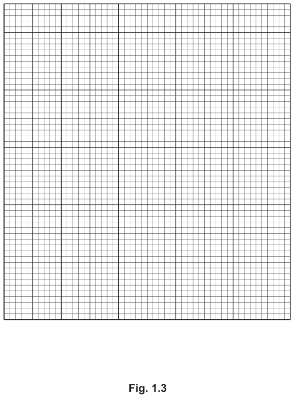
Plot a graph on Fig. 1.3 with the following features:
- x-axis label: concentration of inhibitor /
- x-axis scale: 0.5 to 2.5, marked every 0.5 (i.e. 0.5, 1.0, 1.5, 2.0, 2.5)
- y-axis label: percentage inhibition of sucrase / %
- y-axis scale: 0 to 60, marked every 10 (i.e. 0, 10, 20, 30, 40, 50, 60)
- Points plotted (as small dots in circles or crosses) at: (0.50, 8.0), (1.00, 27.5), (1.50, 44.5), (2.00, 51.0), (2.50, 52.5)
- Points joined by a thin, smooth curve that rises steeply between 0.5 and 1.5 and then levels off (a plateau approaching ~53% at 2.5 )
Use a sharp pencil throughout.
Graph: x-axis 'concentration of inhibitor / mg cm⁻³' (0.5 to 2.5), y-axis 'percentage inhibition of sucrase' (0 to 60%), five points plotted and joined by a smooth curve
Background Concept
A line graph is used to display how a dependent variable (here, percentage inhibition of sucrase) changes with an independent variable (concentration of inhibitor). The independent variable is conventionally placed on the x-axis and the dependent on the y-axis. CIE conventions require:
- A scale that uses at least half the grid in both directions.
- Axis labels that include both the quantity and the unit.
- Points plotted as small dots in circles or crosses (not large blobs) so that the actual point is unambiguous.
- Points joined by a thin line (ruled straight or smooth curve), not by a hand-drawn jagged line.
Understanding the Question
The candidate is asked to plot the data in Table 1.3 on the grid in Fig. 1.3. The data are five (concentration, percentage inhibition) pairs. The expected shape of the curve is a steep rise at low concentrations followed by a plateau as the inhibitor saturates its effect (a typical dose–response curve).
Approach
Choose the x-axis scale to fit the data (0.5 to 2.5 , marked every 0.5) and the y-axis scale to fit the percentage inhibition values (0 to 60%, marked every 10). Plot each of the five points carefully, then join them with a smooth curve that reflects the trend (steep rise, then plateau).
Step-by-Step Reasoning
- The x-axis range is 0.5 to 2.5 . The grid is large enough to accommodate this scale.
- The y-axis range is 0 to 60%. The maximum data value is 52.5%, so 60% gives a small bit of headroom.
- Mark every 0.5 on the x-axis and every 10 on the y-axis. This is the minimum density required by the mark scheme ('labelled at least every 2 cm' of grid).
- Plot each of the five points as a small dot in a circle or a small cross:
- (0.50, 8.0)
- (1.00, 27.5)
- (1.50, 44.5)
- (2.00, 51.0)
- (2.50, 52.5)
- Join the points with a thin, smooth curve. The curve should rise steeply at first (between 0.5 and 1.5 ) and then flatten as it approaches ~53% (between 1.5 and 2.5 ). The point at (2.50, 52.5) is near the top of the plateau.
- Use a sharp pencil so that points and lines are precise and easy to read.
Key Takeaways
- A dose–response curve typically shows a steep rise followed by a plateau as the system approaches saturation.
- Graph conventions: small dots/crosses, thin lines, axes labelled with quantity and unit, scales that use at least half the grid.
- The independent variable (concentration) is on the x-axis; the dependent variable (% inhibition) is on the y-axis.
Common Mistakes
- Labelling the y-axis 'percentage inhibition' without the % sign in the unit.
- Using an awkward scale (e.g. 0.3, 0.6, 0.9, 1.2...) that does not start at 0.5 or does not use half the grid.
- Plotting points as large dots or filled circles, which obscure the exact location.
- Joining the points with straight ruled lines or a hand-drawn jagged line instead of a smooth curve.
- Plotting % inhibition on the x-axis by mistake (the dependent variable goes on the y-axis).
Things to Be Careful About
- The data show a curve, not a straight line: the points must be joined with a smooth curve, not ruled straight lines.
- The y-axis scale should be chosen so the highest data point (52.5%) is well within the grid; 60% is appropriate.
- All five points must be plotted; missing a point loses a mark.
Draw two lines on your graph in Fig. 1.3 to show the concentration of inhibitor that causes 24% inhibition of sucrase.
Answer
On the graph plotted in (b)(i):
- Draw a horizontal dashed line from y = 24% on the y-axis to the point where it meets the curve.
- From that intersection point, draw a vertical dashed line down to the x-axis.
- Read off the concentration of inhibitor at the x-axis. This is the concentration that gives 24% inhibition of sucrase.
Using the graph, the value is approximately .
Horizontal line from y = 24% to the curve, then vertical line down to the x-axis; the x-axis reading is the required concentration of inhibitor (≈ 0.95 mg cm⁻³)
Background Concept
To find an x-value on a graph that corresponds to a given y-value (or vice versa), the standard technique is to draw construction lines. A horizontal line from the y-axis to the curve, followed by a vertical line from the curve to the x-axis, identifies the required (x, y) pair. This works for any smooth curve and is the standard way to interpolate between data points.
Understanding the Question
The candidate has plotted a smooth curve in (b)(i) and now needs to find the concentration of inhibitor that gives exactly 24% inhibition of sucrase. The mark scheme requires that two lines be drawn on the graph: one across from the y-axis, and one down to the x-axis. Both intercepts must be shown.
Approach
Draw a horizontal line from 24% on the y-axis to the curve, then a vertical line from the intersection on the curve down to the x-axis. Read off the x-value.
Step-by-Step Reasoning
- Locate 24% on the y-axis (between the 20 and 30 gridlines, just below halfway).
- Using a ruler, draw a horizontal dashed line from this point across the graph to the right, until it meets the curve.
- From the point of intersection on the curve, draw a vertical dashed line down to the x-axis.
- Read off the x-value where this vertical line meets the x-axis. Using the plotted data, this value lies between 0.5 (where inhibition is 8.0%) and 1.0 (where inhibition is 27.5%). Linear interpolation gives approximately of the way from 0.5 to 1.0, i.e. about .
- The exact value depends on the candidate's plotted curve; the mark scheme only requires that the two construction lines be drawn clearly.
Key Takeaways
- Construction lines (horizontal then vertical) are the standard way to read an x-value from a y-value on a graph.
- The lines should be drawn with a ruler and be clearly visible (dashed lines are conventional).
- The mark scheme credits the lines, not the specific numerical value (which depends on the candidate's plotting).
Common Mistakes
- Drawing the horizontal line in the wrong direction (e.g. starting from the x-axis instead of the y-axis).
- Drawing only one of the two lines (e.g. only the horizontal, leaving the x-value unmarked).
- Drawing the vertical line down to the x-axis but failing to read off the value clearly.
- Drawing the lines freehand (without a ruler) so they are wobbly and the reading is ambiguous.
Things to Be Careful About
- The horizontal line must reach the curve, not stop at the nearest data point (24% does not coincide with any data point, so the line must intersect the curve between two points).
- The vertical line must drop from the point on the curve, not from the nearest data point.
- The lines should be drawn lightly (e.g. dashed) so they do not obscure the plotted curve.
Answer
The inhibitor binds to the enzyme's active site (or to an allosteric site), changing the shape of the active site. This prevents the substrate (sucrose) from binding, reducing the number of enzyme–substrate complexes that can form, and so reducing the rate at which sucrase hydrolyses sucrose into glucose and fructose.
Mark-scheme points covered:
- binds to the enzyme's active site / allosteric site
- changes active site shape
- prevents substrate from binding / formation of enzyme–substrate complexes
- reduces the number of enzyme–substrate complexes
Inhibitor binds to the active site (or allosteric site) of sucrase, changes the shape of the active site, prevents sucrose from binding, reducing the number of enzyme–substrate complexes
Background Concept
Enzymes are biological catalysts with a specific 3D shape, including an active site where the substrate binds. The induced-fit model states that the active site changes shape slightly when the substrate binds, but the resting shape is determined by the enzyme's tertiary structure.
Inhibitors reduce enzyme activity by interfering with this process:
- Competitive inhibitors bind to the active site, competing with the substrate. They directly block the substrate from binding.
- Non-competitive (allosteric) inhibitors bind to a site elsewhere on the enzyme (an allosteric site), changing the shape of the active site so that the substrate can no longer bind effectively.
In both cases, the number of enzyme–substrate complexes that can form per unit time is reduced, and so the rate of reaction falls.
Understanding the Question
The candidate is asked to suggest how the inhibitor from green tea reduces the activity of sucrase. The mark scheme awards up to 2 marks for combining one point from each of two categories:
- Where/how the inhibitor binds (active site or allosteric site)
- The effect on the active site shape and substrate binding
The expected answer combines a binding statement with a consequence statement.
Approach
State that the inhibitor binds (at the active site or at an allosteric site) and that this changes the active site shape, preventing substrate binding and reducing the number of enzyme–substrate complexes.
Step-by-Step Reasoning
- The inhibitor molecule has a shape that is complementary to a region of the sucrase enzyme.
- The inhibitor binds either at the active site (competitive) or at a different (allosteric) site on the enzyme.
- Binding of the inhibitor changes the 3D shape of the active site (in the case of allosteric binding) or directly occupies it (in the case of active-site binding).
- Because the active site no longer fits the substrate (sucrose), fewer enzyme–substrate complexes can form.
- With fewer enzyme–substrate complexes, the rate of hydrolysis of sucrose is reduced, so the activity of sucrase appears lower.
Key Takeaways
- Enzyme inhibitors work by binding to the enzyme (at the active site or an allosteric site) and either blocking the substrate or changing the active site shape.
- The result is a reduction in the number of enzyme–substrate complexes, and therefore a reduced rate of reaction.
- The mark scheme requires both a binding statement AND a consequence statement for full marks.
Common Mistakes
- Vague statements: 'the inhibitor stops the enzyme from working' — does not specify where it binds or how it changes the enzyme.
- Missing the consequence: only stating where the inhibitor binds without saying what happens to substrate binding.
- Confusing the inhibitor with the substrate (e.g. saying the inhibitor is broken down by the enzyme).
- Forgetting to mention that the number of enzyme–substrate complexes is reduced.
Things to Be Careful About
- The question asks for a 'suggestion', so the candidate is not required to commit to whether the inhibition is competitive or non-competitive. Either is acceptable as long as the binding and consequence are stated.
- The key biological terms — 'active site', 'allosteric site', 'enzyme–substrate complex' — should be used precisely.
- The mark scheme awards marks for combining one point from each category; a single point from only one category scores only 1 mark.
The scientists calculated the percentage inhibition of sucrase by measuring the concentration of reducing sugars in the solution after 5 minutes.
Describe how the scientists could determine the concentration of reducing sugars in the solution.
Answer
- Prepare a series of known concentrations of reducing sugar (e.g. glucose) solutions.
- Add Benedict's solution to each known concentration and heat to at least (in a water bath).
- Test the sample in the same way (add Benedict's solution and heat).
- Compare either the time taken to reach a particular colour (e.g. green, yellow, orange, brick red) or the final colour of the sample with the known concentrations; the standard whose colour matches the sample gives the concentration of reducing sugars in the sample.
Mark-scheme points covered:
- prepare known concentrations of reducing sugars
- test known concentrations with Benedict's solution and heat to at least
- test sample with Benedict's and compare, time taken / final colour, to standard / known concentrations
Prepare known concentrations of reducing sugars, add Benedict's solution and heat to at least 80°C, test the sample the same way, and compare the time taken (or final colour) with the standards to determine the concentration
Background Concept
Benedict's reagent (a blue solution containing copper(II) sulfate in an alkaline citrate buffer) reacts with reducing sugars on heating. Cu²⁺ ions are reduced to Cu⁺, which precipitate as red copper(I) oxide. The colour changes from blue to green (low concentration of reducing sugar) to yellow to orange to brick red (high concentration).
To convert this qualitative colour change into a QUANTITATIVE measurement of concentration, a calibration series is needed: a set of standard solutions of known concentration is tested in exactly the same way, and the colour (or the time taken to reach a particular colour) of the unknown sample is compared with the standards.
Understanding the Question
The scientists want to know the concentration of reducing sugars in a solution after 5 minutes of sucrase activity. The candidate is asked to describe how the concentration of reducing sugars could be determined. The mark scheme requires three points:
- A calibration series of known concentrations must be prepared.
- Benedict's solution must be added and the mixture heated to at least 80°C (the temperature at which the reaction proceeds at a useful rate).
- The sample must be compared with the standards using either the time taken to reach a particular colour or the final colour.
Approach
Describe a calibration-based colorimetric procedure: prepare a series of standards, treat each standard identically to the sample (Benedict's + heat), then match the sample's behaviour to the closest standard.
Step-by-Step Reasoning
- Prepare standards: make up a series of solutions of known reducing-sugar concentration (e.g. glucose at 0, 0.5, 1.0, 1.5, 2.0, 2.5 mg cm⁻³). These provide the calibration.
- Treat standards with Benedict's: add a fixed volume of Benedict's reagent to each standard and heat in a water bath at ≥80°C for a fixed time. Observe the colour change (and/or the time taken to reach a particular colour).
- Treat the sample identically: add the same volume of Benedict's reagent to the sample and heat in the same way. Record the final colour (and/or the time taken to reach the same reference colour).
- Compare with the calibration: match the sample's colour (or time) to the standard that gives the same result. The concentration of that standard is the estimated concentration in the sample.
Either the final colour or the time taken to reach a particular colour can be used as the comparison; time is often more reproducible because it is a continuous variable.
Key Takeaways
- Benedict's test on its own is qualitative (it tells you whether a reducing sugar is present, but not how much).
- To make it quantitative, a calibration series of known concentrations is essential.
- Either final colour (a discrete comparison) or time to reach a given colour (a continuous comparison) can be used as the comparison variable.
- Heating to at least 80°C is required for the Benedict's reaction to proceed at a useful rate; below this, the colour change is very slow.
Common Mistakes
- Describing only the qualitative Benedict's test ('add Benedict's, heat, observe the colour change') without mentioning a calibration series.
- Omitting the heating step or specifying an incorrect temperature (e.g. 37°C, which is body temperature and too low).
- Saying 'compare the colour' without specifying what the colour is being compared to (i.e. without mentioning the standards of known concentration).
- Forgetting to use the same volume of Benedict's and the same heating time for the standards and the sample.
Things to Be Careful About
- The comparison must be to STANDARDS of KNOWN concentration — a bare 'compare the colour' is not enough.
- The temperature threshold (≥80°C) is part of the mark scheme; omitting it loses a mark.
- The Benedict's test is for REDUCING sugars, so the procedure is specific to reducing sugars (not all sugars are reducing — sucrose is not, but its hydrolysis products glucose and fructose are).
M1 is a slide of a stained transverse section through a leaf.
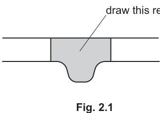
Draw a large plan diagram of the region of the leaf on M1 indicated by the shaded area in Fig. 2.1. Use a sharp pencil.
Use one ruled label line and label to identify the lower epidermis.
Working
A plan diagram shows tissues as outlines, not as individual cells. The conventions to follow are:
- Use a sharp HB pencil; draw thin, continuous lines with no shading.
- Fill most of the space provided.
- Upper epidermis = 3 lines (a single row of cells; the middle line represents the cell-wall layer between adjacent cells seen in section).
- Lower epidermis = 2 lines (the section cuts tangentially through the lower epidermis here, so only two wall layers are seen).
- Mesophyll between the two epidermes is left blank (no individual palisade/spongy cells drawn).
- Vascular bundle: draw with the correct relative size and position, and subdivide it to show xylem and phloem as separate regions.
- Add one ruled label line ending on the lower epidermis; write the label "lower epidermis".
Answer
A large plan diagram of the shaded region: upper epidermis as three parallel lines across the top, lower epidermis as two parallel lines at the bottom, blank mesophyll in between, and a vascular bundle in the central midrib showing subdivisions of xylem (towards the upper side) and phloem (towards the lower side), with a single ruled label line and the label "lower epidermis".
Plan diagram drawn as described; see diagram.
Background Concept
A plan diagram is a low-magnification outline of a specimen that records the shapes, sizes and positions of the different tissues, without showing any individual cells. It is drawn from observation through a microscope and is used to record tissue organisation. Conventions are strict because the diagram is a scientific record: lines must be sharp and continuous, no shading is allowed, and no individual cells may be drawn inside the tissue regions. The number of lines used to represent a single-layered tissue such as an epidermis depends on the orientation of the cut: where the epidermis is cut transversely, two adjacent wall layers are seen as two lines; where a thicker cut is visible, three lines may represent the row of cells plus their bounding walls.
Understanding the Question
You are looking down the microscope at slide M1, a stained transverse section through a leaf. The shaded area in Fig. 2.1 shows the central midrib region that you must draw. You must use a sharp pencil, fill the available space, follow plan-diagram conventions, and add ONE ruled label line to the lower epidermis.
The mark scheme rewards five specific features: using most of the space and drawing the upper epidermis as three lines and the lower epidermis as two; drawing the correct region with no individual cells; the correct proportions of the vascular bundle; subdividing the vascular bundle (to show xylem and phloem); and one correctly placed label on the lower epidermis.
Approach
First, identify the upper epidermis, the lower epidermis, the mesophyll and the vascular bundle. Then plan the size of your drawing so that it fills most of the space (and is large enough to show the bundle subdivisions clearly). Draw the outlines, then check proportions against the slide, and finally add one ruled label.
Step-by-Step Reasoning
- Look at the slide under low power and locate the shaded region from Fig. 2.1. This is the central midrib, with a downward protrusion of the lower epidermis and a flat upper surface.
- Outline the upper epidermis as three lines. The third line represents the cell-wall boundary on the inner side of the cell row; the central line is the shared wall between adjacent epidermal cells.
- Outline the lower epidermis as two lines where the cut passes through the protruding midrib, because only the upper and lower walls of the cells are seen in this region.
- Leave the mesophyll blank — no palisade or spongy mesophyll cells. This is a plan, not a high-power drawing.
- Within the midrib, draw the vascular bundle at the correct size relative to the surrounding tissues. The bundle should be large because it is the main vascular supply of the midrib.
- Subdivide the bundle: xylem towards the upper side, phloem towards the lower side, separated by a thin line representing the cambium/bundle boundary. This earns the "subdivisions" mark.
- Use a sharp pencil; keep all lines thin, continuous and free of shading.
- Add ONE ruled label line that ends exactly on the lower epidermis. Write the label "lower epidermis".
Key Takeaways
- A plan diagram records tissues, not cells: no shading, no internal cell detail.
- The number of lines used to depict a single-cell layer reflects how the section is cut (two lines through the cell, three lines across a row).
- The vascular bundle must be drawn at the correct proportion and must be subdivided.
- Exactly one ruled label line is required; it must touch the structure being labelled.
Common Mistakes
- Drawing individual palisade or spongy mesophyll cells inside the plan (a high-power drawing error, not a plan error).
- Shading the vascular tissue to make it look "solid".
- Drawing the upper and lower epidermis as the same number of lines without checking the section.
- Forgetting to subdivide the bundle, so it appears as one undifferentiated mass.
- Adding more than one label, or using a label that does not end on the structure.
- Using a thick or broken line for any part of the outline.
Things to Be Careful About
The shaded region in Fig. 2.1 is the central midrib, NOT the whole leaf. Only the region indicated should be drawn. Use the available space — a small diagram wastes easy marks. The vascular bundle should look proportionate to the midrib width; an undersized bundle suggests the wrong specimen was examined.
Observe the xylem vessel elements in the leaf on M1.
Select a line of four adjacent xylem vessel elements.
Each xylem vessel element must touch at least one other xylem vessel element.
- Make a large drawing of this line of four xylem vessel elements.
- Use one ruled label line and label to identify the wall of one xylem vessel element.
Working
A high-power drawing of cells is required, not a plan diagram. Conventions:
- Use a sharp pencil; lines must be continuous, thin and sharp, with no shading.
- The cell wall of each xylem vessel element is drawn as TWO close parallel lines (one for each side of the wall), and the two-line wall must be drawn around the entire perimeter of every cell.
- Draw four xylem vessel elements end-to-end in a single line, each one touching at least one other (they should share a wall).
- The shape of xylem vessel elements in transverse section is roughly polygonal/rounded with thickened inner walls; the lumen (empty central space) is clear.
- Add ONE ruled label line that ends on the wall of ONE xylem vessel element; write the label "cell wall" (or equivalent).
Answer
A large drawing of four xylem vessel elements in a line, each touching its neighbour, with each cell wall drawn as a double line all the way around, correct polygonal/rounded shape, and one ruled label line and label to the wall of one cell.
High-power drawing of four xylem vessel elements as described; see diagram.
Background Concept
A high-power (cellular) drawing shows individual cells with their walls and any visible contents. Unlike a plan diagram, individual cells ARE drawn. For a plant cell, the cell wall is shown as TWO close parallel lines (one for each side of the shared wall), and the lines must be continued all the way around the cell. Xylem vessel elements are dead, hollow cells; in transverse section they appear as roughly circular or polygonal outlines with thickened walls and an empty (clear) lumen. They are joined end-to-end, and their end walls are perforated or absent to form continuous vessels.
Understanding the Question
You are looking at slide M1 through the microscope at high power. You must select a line of FOUR adjacent xylem vessel elements (each one must touch at least one other in the line) and draw them large and accurately. You must add ONE ruled label line that ends on the wall of ONE xylem vessel element.
The mark scheme rewards: clean sharp lines with no shading; four correctly selected cells each touching at least one neighbour; a double-line wall drawn around every cell; the correct shape of xylem vessel elements; and one correct label on a cell wall.
Approach
First locate the xylem in the vascular bundle on M1. Choose a row of four elements where each one clearly touches the next. Plan the size of the drawing so the four cells fill most of the available space. Draw each cell with a double-line wall, leave the lumen empty (no contents drawn), and add one label.
Step-by-Step Reasoning
- Centre the xylem in the field of view and choose a clean line of four xylem vessel elements. They should form a single row, each touching the next along a shared wall.
- Plan the size of the drawing so the four cells together fill most of the available space, but cells should not overlap or run off the page.
- Draw the outline of the first cell as two close parallel lines, then continue around the whole cell so the wall is a complete double line.
- Where the second cell touches the first, the double-line wall of the first cell is also the double-line wall of the second; do not draw extra lines for the shared wall.
- Repeat for the third and fourth cells, so all four cells have a complete double-line wall and they all touch.
- Xylem vessel elements have a roughly polygonal/rounded outline with thickened walls and an empty lumen — do not shade the wall or fill the lumen.
- Add ONE ruled label line that ends exactly on the wall of one xylem vessel element. Write the label "cell wall".
- Check: lines continuous and thin, no shading, four cells each touching a neighbour, double-line wall around each, correct shape, one correct label.
Key Takeaways
- A cell drawing is fundamentally different from a plan diagram: cells ARE drawn, but the contents (here, lumen) are not shaded.
- Every cell wall in a cell drawing is shown as TWO close parallel lines, all the way around the cell.
- The chosen cells must be a connected line of four, each touching at least one neighbour — isolated cells do not earn the mark.
- Only one label is required and it must end on the structure named.
Common Mistakes
- Drawing single-line walls (this is a plan-diagram error carried over).
- Shading the wall or filling the lumen (xylem vessel elements are empty when mature).
- Drawing the four cells but not in a single line, or with one cell not touching a neighbour.
- Adding multiple labels, or writing a label that does not end on a wall.
- Drawing cells that are too small, or letting them overlap or run off the page.
Things to Be Careful About
The label line must be a straight ruled line that ends ON the wall, not floating in the lumen or pointing into the empty space. The drawing must be done at high power so the cells are large enough to show the wall as two lines clearly. Do not include companion cells, parenchyma or any other cell type in the line; only xylem vessel elements count for this mark.
Fig. 2.2 shows a photomicrograph of a transverse section through a different leaf from that on M1.
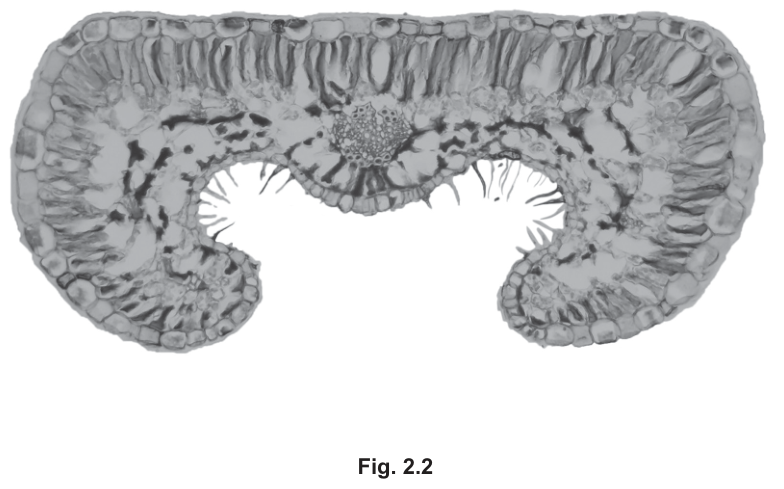
Identify three observable differences, other than colour, between the section on M1 and the section in Fig. 2.2.
Record these three observable differences in Table 2.1.
Table 2.1
| feature | M1 | Fig. 2.2 |
|---|---|---|
Answer
| feature | M1 | Fig. 2.2 |
|---|---|---|
| number of vascular bundles | more | fewer |
| size of vascular bundles | larger | smaller |
| presence of trichomes (hairs) | absent | present |
| shape of leaf | straight | curled |
Any three of the four paired differences above earn the three content marks; the fourth mark is for recording the differences in a correctly structured table.
Three observable differences recorded in the table, e.g. number/size of vascular bundles, presence of trichomes, leaf shape.
Background Concept
When comparing two specimens under the microscope (or two photomicrographs), the marks go only to OBSERVABLE features — things you can actually see in the image or down the microscope. Inferences such as "xylem is lignified" or "this is from a xerophyte" are NOT observable and so do not earn marks here. Differences must be paired across the two specimens, with one observation per specimen, and recorded clearly in a table.
Understanding the Question
You have slide M1 (a leaf transverse section you are observing) and Fig. 2.2 (a photomicrograph of a different leaf's transverse section). You must identify three observable differences (other than colour) between them, and record them in Table 2.1 as paired entries.
The mark scheme credits any three of: number of vascular bundles, size of vascular bundles, presence/absence of trichomes, and shape of the leaf. The fourth mark is awarded for correctly presenting these in the table.
Approach
Look at M1 through the microscope and at the printed Fig. 2.2 side by side. For each of the credited features, decide what is observable in M1 and what is observable in Fig. 2.2. State each difference as a paired entry, with the M1 observation in the second column and the Fig. 2.2 observation in the third. Stick to what is directly visible.
Step-by-Step Reasoning
- Vascular bundles — number. In M1, scan the section under low power and count the vascular bundles in the lamina. In Fig. 2.2, the visible bundle(s) are few — typically only the central midrib bundle is clearly shown.
- Vascular bundles — size. Compare the size of the largest vascular bundle in M1 with the size of the bundle in Fig. 2.2. The bundles in M1 are large (they include a prominent midrib bundle); the bundles in Fig. 2.2 are small.
- Trichomes (hairs). In M1, look at both surfaces of the leaf. No hairs are present. In Fig. 2.2, distinct hair-like projections (trichomes) are clearly visible on the inner (concave) surface of the curled leaf.
- Leaf shape. In M1, the leaf section is straight (the laminae on either side of the midrib are flat). In Fig. 2.2, the leaf is curled inwards to form a C-shape, with a clear gap between the two ends.
- Enter the chosen three (or four) paired differences into Table 2.1, one observation per cell, no extra text in the table.
Key Takeaways
- Only OBSERVABLE features count. Phrases like "more xylem" or "drier habitat" do not earn marks unless they describe what is visible.
- Differences must be paired: a feature about M1 alongside the same feature about Fig. 2.2.
- Avoid colour — the question explicitly rules it out.
- A well-set-out table earns its own mark, independent of the content marks.
Common Mistakes
- Writing inferences (e.g. "Fig. 2.2 is a xerophyte", "M1 has more chloroplasts") rather than what can be seen.
- Listing differences without pairing them across the two columns.
- Repeating the same feature under two rows (e.g. "more bundles" and "larger bundles") when only the count is observable in some cases.
- Writing a statement instead of a paired difference (e.g. "M1 is straight" alone).
- Stating a colour difference (explicitly excluded by the question).
Things to Be Careful About
Both specimens must be looked at carefully. The leaf in Fig. 2.2 is unusual because it is curled inwards; many students do not register the C-shape as a shape difference and miss an easy mark. Trichomes may be called "hairs"; either is acceptable provided it is observable. Counting vascular bundles should be done at low power so the whole section is in view.
Fig. 2.3 is the same photomicrograph as that shown in Fig. 2.2.
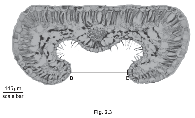
Use the scale bar on Fig. 2.3 and the line D–E to calculate the actual length of the gap between the ends of the leaf.
Show your working, including units and give your answer in micrometres (µm).
actual length of gap = ______
Working
Measure the length of the scale bar and the length of the line D–E on Fig. 2.3 in the same units (e.g. mm with a ruler).
Representative example (values depend on the candidate's own measurement):
- Measured length of scale bar =
- Measured length of D–E =
Answer
actual length of gap ≈ (representative value; the candidate's own measurement will determine the precise number, which will typically be in the range –).
≈ 363 µm (representative; based on a measured D–E length of 50 mm against a 20 mm scale bar representing 145 µm).
Background Concept
A photomicrograph often carries a scale bar — a small line of known real-world length printed on the image. The scale bar can be used to find the actual size of any other feature in the same image, because the magnification is uniform across the image. The relationship is:
The measured sizes must be in the SAME units because they cancel in the ratio. The final answer must be quoted in the units requested (here, micrometres, µm) and to a sensible number of significant figures (usually 2–3 for this type of measurement).
Understanding the Question
Fig. 2.3 is the same photomicrograph as Fig. 2.2 but with a scale bar of and a line D–E drawn between the two curled ends of the leaf. You must measure both lengths on the printed image, set up the proportion, and calculate the actual length of the gap D–E in micrometres. The mark scheme awards four marks: stating the scale-bar length and units, stating the measured D–E length and units, showing the calculation (D–E / scale bar × 145 µm), and stating the final answer.
Approach
Take a ruler and measure the printed length of the scale bar in mm, then measure the printed length of the D–E line in mm. Divide the D–E length by the scale-bar length and multiply by 145 µm. Quote the final answer in µm.
Step-by-Step Reasoning
- Identify the scale bar on Fig. 2.3. It is labelled . State this value with its unit for mark 1.
- Using a ruler, measure the printed length of the scale bar. (The mark scheme credits stating the measured length with an appropriate unit such as mm.)
- Using the same ruler, measure the printed length of the line D–E between the two ends of the leaf. State this measured length with its unit for mark 2.
- Set up the proportion for mark 3:
- Substitute the values and evaluate. In the representative example, .
- Quote the final answer in µm (mark 4). A reasonable number of significant figures is 3 (e.g. or ), reflecting the precision of the measurement.
Because the printed D–E line is approximately 2.5 scale-bar lengths long, any correct measurement by the candidate will give an answer close to , so the expected range is roughly –.
Key Takeaways
- A scale bar allows the actual size of any feature on the same image to be calculated by proportion.
- The two lengths used in the ratio must be in the SAME units; they cancel out.
- Always state the scale-bar value and your measured lengths with units, and show the calculation explicitly.
- The final answer must be quoted in the unit the question asks for (here, µm).
Common Mistakes
- Forgetting to state the scale-bar value with its unit (145 µm), or stating the wrong value.
- Mixing units in the ratio (e.g. dividing a length in cm by a length in mm without converting).
- Omitting the calculation step, just writing a final number.
- Quoting the answer in mm or cm instead of µm.
- Over-quoting significant figures (e.g. 362.500 µm) when the measurement supports only 2–3.
- Dividing the wrong way round (dividing the scale bar by D–E instead of D–E by the scale bar).
Things to Be Careful About
The scale bar is a PRINTED line on the photomicrograph; it does not change with the magnification at which you view the image. Measure both lengths with the same ruler, in the same orientation, and to the nearest mm. The D–E line is horizontal; hold the ruler parallel to it. The answer depends on the candidate's own measurement and so will vary by a few µm; this is normal and accepted.