Biology 9700/35 — May/June 2025
Cambridge AS Level · Advanced Practical Skills · worked solutions for every part, with the mark scheme
Topics Presentation of Data and Observations · Manipulation, Measurement and Observation · Analysis, Conclusions and Evaluation · Use of the Light Microscope
Catalase is an enzyme found in plant tissues. It catalyses the breakdown of hydrogen peroxide, releasing oxygen gas.
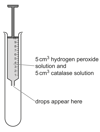
When a mixture of catalase and hydrogen peroxide is put into a syringe, oxygen gas is produced and drops of the mixture come out of the nozzle of the syringe.
You will investigate the effect of different concentrations of catalase on the breakdown of hydrogen peroxide.
You are provided with the materials shown in Table 1.1.
Table 1.1
| labelled | contents | hazard | volume / |
|---|---|---|---|
| E | 100.0% catalase solution | irritant | 50 |
| H | hydrogen peroxide solution | irritant | 30 |
| W | distilled water | none | 100 |
If any solution comes into contact with your skin, wash off immediately under cold water.
You should wear suitable eye protection.
You will need to make different concentrations of the catalase using proportional dilution of the 100.0% catalase solution, E.
You will need to prepare of each concentration, using E and W.
Table 1.2 shows how to prepare two of the concentrations of catalase you will use.
Decide which other concentrations of catalase you will use.
Complete Table 1.2 for the other concentrations you will use.
Table 1.2
| percentage concentration of catalase | volume of E / | volume of W / |
|---|---|---|
| 100.0 | 20.0 | 0.0 |
| 0.0 | 0.0 | 20.0 |
Answer
| percentage concentration of catalase | volume of E / | volume of W / |
|---|---|---|
| 100.0 | 20.0 | 0.0 |
| 75.0 | 15.0 | 5.0 |
| 50.0 | 10.0 | 10.0 |
| 25.0 | 5.0 | 15.0 |
| 0.0 | 0.0 | 20.0 |
75%: 15.0 cm³ E + 5.0 cm³ W; 50%: 10.0 cm³ E + 10.0 cm³ W; 25%: 5.0 cm³ E + 15.0 cm³ W
Background Concept
Proportional (or simple) dilution is the standard laboratory technique for preparing a range of solutions of known concentration from a single stock. The underlying relationship is:
where and are the concentration and volume of the stock, and and are the concentration and total volume of the diluted solution. Equivalently, the volume of stock required is:
and the volume of diluent (W) is whatever is needed to make the total volume up. The two volumes must therefore always sum to the required total.
Understanding the Question
The 100% catalase stock (E) and distilled water (W) are mixed in a beaker to give of each concentration. The 100.0% and 0.0% rows are already filled in. You need to add at least three intermediate concentrations, with the correct volume of E and the correct volume of W for each, so that the pair of volumes sums to .
Approach
Pick intermediate concentrations that are evenly spaced and easy to measure. A common CIE choice is 25%, 50% and 75%, because each of those makes the volume of E numerically equal to a multiple of 5 cm³, which is convenient to draw up with a 10 cm³ graduated pipette or syringe. For each chosen concentration, take the same percentage of as the volume of E, and make the volume of W up to .
Step-by-Step Reasoning
- Choose 25%, 50% and 75% as the three intermediate concentrations — evenly spaced and using round volumes.
- For 75%: of E; W = .
- For 50%: of E; W = .
- For 25%: of E; W = .
- Each pair of volumes must sum to exactly — check.
Key Takeaways
- Proportional dilution: (where is expressed as a decimal fraction).
- Choose evenly spaced intermediate concentrations so the trend is clear and the volumes are easy to measure.
- Always check that the volumes of stock and diluent sum to the required total.
Common Mistakes
- Using awkward percentages (e.g., 33% / 67%) that make volumes hard to measure accurately.
- Forgetting to make the volumes sum to (a common slip is putting 4.5 cm³ + 15.5 cm³ for 22.5%).
- Not providing at least three intermediate concentrations — the mark scheme explicitly requires this.
Things to Be Careful About
- Use a graduated pipette or syringe accurate to or better to measure each volume.
- Label each beaker clearly with the percentage concentration to avoid mix-ups when the same syringe is reused.
- The 0% control (water only) is important — it shows that any reaction observed depends on the enzyme, not on spontaneous decomposition of H₂O₂.
Carry out step 1 to step 8.
step 1 In the beakers provided, prepare the concentrations of catalase as shown in Table 1.2.
step 2 Label large test-tubes with the concentrations of catalase prepared in step 1.
step 3 Fill a syringe to the mark with hydrogen peroxide solution, H.
step 4 Fill the same syringe to the mark with the 100.0% catalase solution.
step 5 Place the syringe in the large test-tube labelled 100.0%, as shown in Fig. 1.1.
step 6 Start the timer.
step 7 Count the number of drops produced in 60 seconds. Record your results in (a)(ii).
step 8 Repeat step 3 to step 7 using the other concentrations of catalase prepared in step 1.
Record your results in an appropriate table.
Answer
| percentage concentration of catalase | number of drops |
|---|---|
| 100.0 | 60 |
| 75.0 | 50 |
| 50.0 | 35 |
| 25.0 | 20 |
| 0.0 | 0 |
(Representative values: the number of drops in increases as the catalase concentration increases. The 0% control produces 0 drops.)
Representative results: ~60, 50, 35, 20, 0 drops for 100%, 75%, 50%, 25%, 0% catalase respectively
Background Concept
Recording experimental results in a properly formatted table is a Paper 3 skill that earns marks for conventions, not for the absolute numbers. The key conventions are:
- The independent variable (what is changed) goes in the left column.
- The dependent variable (what is measured) goes in the right column.
- Each column heading has the quantity and its unit (no units in the data cells).
- Data are recorded to a consistent level of precision — for countable objects (drops), this is a whole number.
The CIE mark scheme gives separate marks for the IV heading, the DV heading, the data, the expected trend, and the use of whole numbers. Each is a discrete skill, so a strong candidate attends to all of them.
Understanding the Question
The procedure in steps 1–8 is set up: in Fig. 1.1, the syringe contains a mixture of hydrogen peroxide solution and catalase solution, with the nozzle pointing down into a large test-tube. As the catalase breaks down the H₂O₂, oxygen gas builds up inside the syringe and pushes the liquid out of the nozzle as drops. You count how many drops fall in for each of the five catalase concentrations and record the counts in a results table. The 0% control (water only) acts as a check that any gas produced is from the catalase reaction and not from spontaneous decomposition of H₂O₂.
Approach
Draw a results table with two columns: the catalase concentration on the left (IV) and the number of drops on the right (DV). Record the data for all five concentrations. Counts are in whole numbers. The expected trend is that higher catalase concentration gives more drops, because more enzyme means more active sites are available (this is the explanation you give in (a)(iv)).
Step-by-Step Reasoning
- The independent variable is the percentage concentration of catalase — this is what is changed between trials, so it goes in the left column.
- The dependent variable is the number of drops produced in — what is measured, so it goes in the right column.
- For each concentration, the count is taken over using the apparatus in Fig. 1.1. A representative set of values is 60, 50, 35, 20, 0 for 100%, 75%, 50%, 25%, 0% catalase respectively. Your own results will vary but the trend should be clear: more catalase, more drops.
- The 0% row should give 0 drops (or very close to 0): the reaction cannot proceed without the enzyme.
- All counts are whole numbers — a 'drop' is a discrete event and you cannot have half a drop.
Key Takeaways
- Table headings: quantity with unit, no units in the cells.
- IV on the left, DV on the right.
- Countable data → whole numbers.
- The 0% control confirms that the gas comes from the enzyme-catalysed reaction.
Common Mistakes
- Putting the unit in the data cells instead of the heading (e.g., writing '60 drops' in the cell rather than 'number of drops' in the heading).
- Reversing IV and DV (concentration on the right, drops on the left).
- Recording a value like '35.5' for a drop count — drops are whole numbers.
- Forgetting to record the 0% control.
- Recording the average of several trials without first recording the individual counts (the mark scheme rewards raw data, not a summary).
Things to Be Careful About
- Wash and dry the syringe between trials to avoid carry-over of catalase, which would inflate the count for the next, lower concentration.
- Start the timer only once the syringe nozzle is in place and the reaction has just begun — otherwise the first few drops may be missed (this is one of the sources of error in (a)(vii)).
- The total volume in the syringe is for every trial — only the catalase concentration changes.
Answer
The greater the concentration of catalase, the more drops are produced in .
As catalase concentration increases, the number of drops produced in 60 s increases.
Background Concept
A 'trend' is a one-sentence summary of how the dependent variable changes as the independent variable is increased. It should describe the direction of the change (increasing, decreasing, no change) and, where appropriate, the shape (linear, curved, plateauing). It does not explain why — that is a separate 'explain' question.
Understanding the Question
You are asked to describe the pattern in YOUR results from (a)(ii). The mark scheme accepts any wording that captures the positive correlation between catalase concentration and number of drops, e.g. 'the higher the concentration of catalase, the more drops'.
Approach
Look at your results table. The first column increases (0% → 100%) and the second column also increases (0 → ~60). State this relationship in a single sentence, starting with the IV and finishing with the DV. Do not give numerical values unless the trend is non-linear (e.g., 'levels off') — for a simple positive trend, a single sentence is enough.
Step-by-Step Reasoning
- The IV is catalase concentration; the DV is number of drops.
- From the table, both increase together. So the trend is positive: 'as catalase concentration increases, number of drops increases'.
- A concise, mark-scheme-matching statement: 'The greater the concentration of catalase, the more drops are produced in .'
- No explanation is needed here — that is what (a)(iv) is for. Do not write 'because there are more active sites' — that is explanation, not description, and would be a misread of the command word.
Key Takeaways
- A trend statement names both variables and the direction of change.
- It should be one or two sentences, not a paragraph.
- It does not need to use the word 'trend' itself.
Common Mistakes
- Stating only one of the two variables (e.g., 'concentration of catalase increases' without mentioning drops).
- Explaining the trend rather than describing it (e.g., 'because there are more active sites' is explanation, not description).
- Adding unnecessary numerical detail when a simple statement will do.
- Saying the trend is linear when the data are clearly curved (here, the differences between successive rows are not constant).
Things to Be Careful About
- Quote your own results, not a generic textbook trend — the mark scheme accepts wording 'according to the candidate's results'.
- Use the command word 'describe', not 'explain' — leave the mechanism for (a)(iv).
Use your results in (a)(ii) to explain the effect of catalase concentration on the breakdown of hydrogen peroxide.
Answer
- As the concentration of catalase increases, there are more active sites available for the hydrogen peroxide substrate to bind to.
- This increases the number of enzyme–substrate complexes formed per unit time, so more oxygen is produced and more drops are released in .
More catalase provides more active sites; this increases the number of enzyme–substrate complexes formed per unit time, raising the rate of oxygen production.
Background Concept
Enzymes are biological catalysts that work by binding their substrate at a specific region called the active site, forming an enzyme–substrate (ES) complex. The complex then breaks down to release the product(s) and regenerate the free enzyme. The rate of the catalysed reaction therefore depends on how often ES complexes form per unit time.
When the enzyme concentration is the limiting factor (i.e., substrate is in excess), the rate of reaction is directly proportional to the number of active sites available. More enzyme molecules → more active sites → more chance of an enzyme–substrate collision → more ES complexes per second → faster product formation.
In this experiment, hydrogen peroxide is in large excess (5 cm³ of a high-concentration stock vs. 5 cm³ of catalase), so the rate is limited by catalase concentration. As catalase concentration rises, the rate at which H₂O₂ is broken down to water and oxygen rises, so oxygen gas pushes the syringe contents out faster, producing more drops in the fixed 60-second period.
Understanding the Question
You are asked to explain — not just describe — the trend seen in your (a)(ii) results, using the underlying biology of enzyme action. The mark scheme requires two specific points:
- Higher catalase concentration → more active sites available.
- More active sites → more enzyme–substrate complexes formed per unit time.
Approach
Link the independent variable (catalase concentration) to the dependent variable (number of drops) through the causal chain:
Make sure each step in the chain is biologically justified.
Step-by-Step Reasoning
- More enzyme molecules at higher concentration: A more concentrated solution contains more catalase molecules per unit volume. Each molecule carries one active site, so the total number of active sites in the syringe is greater.
- More active sites → more ES complexes per unit time: With more active sites available, more hydrogen peroxide molecules can be bound and broken down per second. The number of ES complexes formed per unit time is higher, so the rate of oxygen production is higher.
- Link to the data: More oxygen in 60 s pushes more liquid out of the syringe nozzle, so more drops are counted.
Key Takeaways
- The 'active site' idea is the mechanistic link between enzyme concentration and rate.
- 'ES complex' is the precise CIE term — not 'collision' or 'reaction'.
- When substrate is in excess, the rate is limited by enzyme concentration.
Common Mistakes
- Saying 'more catalase means a faster reaction' without explaining the mechanism (no active site / ES complex language).
- Talking about 'more collisions' rather than 'more ES complexes' — collisions are necessary but it is the formation of the complex that allows the reaction to proceed.
- Confusing enzyme concentration with substrate concentration.
- Saying the enzyme 'makes' the reaction happen — enzymes lower the activation energy, they do not 'create' reactions.
Things to Be Careful About
- The exact phrasing 'enzyme–substrate complex' is the mark scheme's term; alternatives like 'enzyme–substrate binding' are usually accepted, but 'complex' is the precise wording.
- Do not state that 'the reaction is faster' without justifying it with the active-site argument.
Answer
Concentration of catalase (percentage concentration of catalase).
Concentration of catalase
Background Concept
In any experiment there are three categories of variable:
- Independent variable (IV): what the experimenter deliberately changes between trials.
- Dependent variable (DV): what is measured to see the effect of the IV.
- Controlled variables: everything else that must be kept the same so the IV is the only thing affecting the DV.
Understanding the Question
The procedure varies the catalase concentration between trials (100% → 75% → 50% → 25% → 0%) and measures the resulting number of drops. The IV is therefore the catalase concentration.
Approach
Ask: 'What did I deliberately change from one trial to the next?' The answer is the catalase concentration.
Step-by-Step Reasoning
- The IV is the variable whose value the experimenter sets. In this investigation, the experimenter decides whether to test 100%, 75%, 50%, 25% or 0% catalase. That is the IV.
- The mark scheme accepts 'catalase concentration' (or the longer form 'percentage concentration of catalase').
Key Takeaways
- IV = the variable that is changed on purpose.
- DV = the variable that is measured.
- Control variables are kept constant; this is the topic of (a)(vi).
Common Mistakes
- Naming the DV ('number of drops') by mistake.
- Naming a controlled variable (e.g., 'time', 'volume of H₂O₂').
- Stating 'catalase' alone — the mark scheme requires the word 'concentration' (or 'amount' / 'percentage').
Things to Be Careful About
- 'Concentration' is the specific term the mark scheme expects; 'amount' is acceptable but 'volume' is not (because 'volume' refers to a controlled variable in this investigation).
Answer
Any one of:
- volume of catalase ()
- volume of hydrogen peroxide ()
- concentration of hydrogen peroxide
- time ()
Volume of hydrogen peroxide (or volume of catalase / concentration of H₂O₂ / time)
Background Concept
A controlled variable is anything other than the IV and DV that could affect the outcome, and is therefore deliberately kept the same for every trial. Failing to control a relevant variable makes it impossible to attribute any change in the DV to the IV with confidence.
Understanding the Question
The mark scheme accepts any one of four specific controlled variables that the procedure in this investigation holds constant. You need to name just one of them.
Approach
Read through steps 3–8 and identify a quantity that is the same for every concentration. The candidates are:
- Volume of catalase — drawn up in every trial (step 4).
- Volume of hydrogen peroxide — drawn up in every trial (step 3).
- Concentration of hydrogen peroxide — the same stock H is used throughout.
- Time — drops are counted over in every trial (step 7).
Step-by-Step Reasoning
- Each of the four is held constant by the written procedure. Naming any one earns the mark.
- The most obvious answer is time (), because it is stated explicitly in step 7.
- Volume of hydrogen peroxide and volume of catalase are also defensible — the procedure uses of each in every trial.
- Concentration of hydrogen peroxide is valid because the same stock bottle of H is used throughout.
Key Takeaways
- A controlled variable is anything the procedure keeps the same so the IV is the only thing that changes the DV.
- Any single, defensible controlled variable is sufficient for the mark.
Common Mistakes
- Stating the IV ('catalase concentration') — the question asks for a constant.
- Stating the DV ('number of drops') — that is what is measured, not held constant.
- Naming a variable that does change between trials (e.g., 'syringe size' — only one syringe is used, but the procedure doesn't explicitly say so).
Things to Be Careful About
- 'Time' must be qualified — the mark scheme accepts 'time' as shorthand for 'the duration over which drops are counted'.
Answer
Any two of:
- Drops may already have started forming before the timer was started.
- Drop size varies, so a 'drop' is not a fixed volume — different-sized drops affect the count.
- Drops come out too fast to count accurately, especially at high catalase concentrations.
(2 marks: 1 for each correctly identified source of error.)
Any two of: drops formed before timing started / drop size varies / drops too fast to count accurately
Background Concept
A source of error is a specific weakness in the procedure or equipment that makes the recorded value unreliable. For Paper 3, the mark scheme lists the errors it accepts; you should give the specific reason rather than a vague 'human error' or 'parallax'.
Understanding the Question
Step 7 says: 'Start the timer. Count the number of drops produced in 60 seconds.' The two marks are for two distinct, specific problems with this counting step.
Approach
For each mark, ask: 'What could go wrong while counting drops at the tip of a syringe?' The mark scheme lists three credible issues; any two of them earn the marks.
Step-by-Step Reasoning
- Drops already being produced before timing starts: the reaction begins the instant catalase and H₂O₂ are mixed, and the syringe is filled before the timer is started. By the time the nozzle is positioned over the test-tube and the timer pressed, several drops may already have fallen. This systematically underestimates the count for the faster (higher-concentration) trials.
- Drop size varies: a 'drop' is not a calibrated unit. Surface tension, the shape of the nozzle tip, and the pressure inside the syringe all affect drop size, so two 'drops' may contain different volumes of gas. This means the count is not a true measure of the volume of oxygen released.
- Drops too fast to count accurately: at high catalase concentrations, drops fall faster than one can be reliably counted. A 10-drop/second stream is easy to miscount by 2–3 drops in 60 s. This introduces random error that grows with the rate.
Key Takeaways
- A 'source of error' must be specific to the procedure, not a generic 'human error'.
- Each error must affect the measured value, and the way it does so should be stated.
- Two distinct errors are required, not the same error phrased twice.
Common Mistakes
- Vague answers such as 'human error', 'parallax error', 'misreading the timer' — these are too generic to earn marks.
- Restating the same error twice ('drops formed before timing started' and 'drops formed too early').
- Naming an error that is not in step 7 (e.g., 'concentration of H₂O₂ might change' — the procedure does not vary it).
- Listing 'inaccurate measuring cylinder' — no measuring cylinder is used in step 7.
Things to Be Careful About
- The errors are about step 7 specifically — the counting step, not the whole procedure.
- The mark scheme phrasing is specific: 'drops already started being produced', 'drop size varies', 'drops too fast to count accurately'.
Describe how you would modify the procedure to investigate the effect of substrate concentration on catalase activity.
Answer
- Use five different concentrations of hydrogen peroxide (e.g., prepared by proportional dilution of the stock H) instead of five concentrations of catalase.
- Keep the concentration of catalase the same (e.g., 100% catalase) for every trial.
(All other steps — volumes, time, apparatus — remain unchanged.)
Use five different concentrations of H₂O₂ and keep the catalase concentration constant (e.g., 100%) for every trial.
Background Concept
To investigate the effect of substrate concentration on enzyme activity, the substrate (here, hydrogen peroxide) becomes the new independent variable, and the enzyme (catalase) becomes the new controlled variable. Everything else in the procedure — volumes, time, apparatus — is held constant, just as in the original investigation.
Understanding the Question
The mark scheme requires two specific changes to the procedure in steps 1–8:
- The new IV: five different concentrations of hydrogen peroxide.
- The constant: the same concentration of catalase for every trial (e.g., 100% catalase E).
Approach
Re-read the original procedure and ask: 'What has to change so that substrate concentration is the new IV?' Then ask: 'What new variable must be kept constant so that the substrate is the only thing affecting the rate?'
Step-by-Step Reasoning
- New IV — five concentrations of H₂O₂: prepare these by proportional dilution of the stock H using distilled water W (e.g., 100%, 75%, 50%, 25%, 0% of H, each made up to a fixed total volume). The same five-concentration pattern as in (a)(i) is a good template.
- Constant — one catalase concentration: use 100% catalase (E) for every trial. The catalase is now the controlled variable, not the IV.
- The remaining steps (volumes, time, apparatus) are unchanged. The rate of oxygen production (number of drops in 60 s) is still the DV.
Key Takeaways
- Swapping IV and DV is a standard modification: what was the IV becomes a control, and vice versa.
- The number of concentrations (≥5) and the use of a 0% control (e.g., water only) are preserved.
- The same proportional-dilution technique is used to make the new series of substrate concentrations.
Common Mistakes
- Saying 'change the catalase' — that is what the original procedure already does.
- Forgetting to specify the number of concentrations — the mark scheme requires 'five different'.
- Varying both H₂O₂ and catalase at the same time, which makes it impossible to attribute the effect to either.
- Forgetting to keep the catalase concentration constant — the second mark is for this explicit statement.
Things to Be Careful About
- The 0% H₂O₂ control is still needed — it confirms that any gas produced comes from the catalase–H₂O₂ reaction.
- The 0% control in the new series would be 0% H₂O₂ (= 100% W), and the rate here should be zero.
The catalase activity of germinating hyacinth seeds was measured when the seeds were placed in different concentrations of salt solution.
Table 1.3 shows the results of the investigation.
Table 1.3
| concentration of salt solution / | catalase activity / arbitrary units |
|---|---|
| 0 | 72 |
| 100 | 35 |
| 200 | 28 |
| 300 | 23 |
| 400 | 20 |
| 500 | 14 |

Answer
Plot the data on the grid in Fig. 1.2 as follows:
- X-axis: concentration of salt / ; scale 100 to 2 cm (e.g., 0 to 600, with labels every 200).
- Y-axis: catalase activity / arbitrary units; scale 20 to 2 cm (e.g., 0 to 80, with labels every 20).
- Points (small dots in circles or crosses): (0, 72), (100, 35), (200, 28), (300, 23), (400, 20), (500, 14).
- Line: a thin smooth curve passing through all six points — steep drop from (0, 72) to (100, 35), then a more gradual decline.
Graph with x-axis 'concentration of salt / mmol dm⁻³' (scale 100 to 2 cm), y-axis 'catalase activity / arbitrary units' (scale 20 to 2 cm), six points joined by a thin smooth curve through all points
Background Concept
A line graph is used when both the independent and dependent variables are continuous numerical data, and the relationship between them is being investigated. CIE conventions for plotting include:
- X-axis: independent variable (the one the experimenter set).
- Y-axis: dependent variable (the one measured).
- Labels: each axis has a quantity and unit (e.g., 'concentration of salt / ').
- Scales: linear, using at least half the grid in both directions, with the interval being a convenient number (1, 2, 5, 10, etc., not 3, 7, etc.).
- Points: plotted precisely as small dots in circles or as small crosses.
- Line: a thin smooth curve passing through (or as close as possible to) all points — not dot-to-dot straight segments if the data are clearly curved, and not a forced straight line of best fit unless the relationship is linear.
Understanding the Question
You are given six data points showing how catalase activity in germinating hyacinth seeds changes with salt concentration. You must plot these on the provided grid (Fig. 1.2) following the conventions above. Four marks are available: one for axis labels, one for scales, one for accurate plotting, and one for the smooth line.
Approach
- Decide the IV and DV: IV = salt concentration, DV = catalase activity. Place them on the x- and y-axes respectively.
- Choose scales that use at least half the grid and have convenient intervals. The mark scheme specifies 100 per 2 cm on the x-axis and 20 per 2 cm on the y-axis.
- Label both axes with quantity and unit.
- Plot each of the six points as a small dot in a circle or as a small cross.
- Join the points with a thin smooth curve passing through all six.
Step-by-Step Reasoning
- X-axis: 'concentration of salt / '. Data range 0–500. Using 100 to 2 cm, the axis can run from 0 to 600 in 12 cm (or 0 to 500 in 10 cm). Either uses at least half the grid. Label every 2 cm, so every 200 units: 0, 200, 400, 600 (or 0, 200, 400).
- Y-axis: 'catalase activity / arbitrary units'. Data range 14–72. Using 20 to 2 cm, the axis can run from 0 to 80 in 8 cm. Label every 2 cm, so every 20 units: 0, 20, 40, 60, 80.
- Plot the six points:
- (0, 72)
- (100, 35)
- (200, 28)
- (300, 23)
- (400, 20)
- (500, 14)
- Join with a thin smooth curve passing through all six points. The shape: a steep drop from (0, 72) to (100, 35), then a more gradual decline that flattens as salt concentration increases.
Key Takeaways
- IV on x, DV on y.
- Scales must use at least half the grid with convenient intervals.
- Always include units in the axis label, separated by '/'.
- Use small dots in circles or small crosses for points — not large blobs.
- A smooth curve through all points; not straight dot-to-dot segments.
Common Mistakes
- Forgetting the unit on the x-axis label ('').
- Using an awkward scale (e.g., 30 to 1 cm) that does not allow accurate plotting.
- Plotting points as large filled dots, which makes them hard to read.
- Drawing a forced straight line of best fit — the relationship is clearly curved, not linear.
- Not extending the axis to include all data (e.g., ending the y-axis at 70 when the highest point is 72).
Things to Be Careful About
- The mark scheme specifies 'small dots in circles or crosses' — large filled dots lose marks.
- The line should be thin and continuous, not a series of disjointed segments.
- The y-axis should start at 0; the x-axis should also start at 0 unless there is a clear reason not to.
A germinating hyacinth seed was placed in a salt solution of unknown concentration. The catalase activity was found to be 54 arbitrary units.
Estimate the concentration of salt solution at which the seed was germinated.
Show on your graph how you obtained your estimate.
concentration = ______
Working
- On the y-axis, mark a horizontal line at catalase activity = 54 arbitrary units.
- Draw this line across to where it meets the curve.
- From the intersection, drop a vertical line down to the x-axis.
- Read off the concentration of salt at this point.
The estimated concentration is approximately 45–50 (typical Cambridge answer: ≈ 50 ).
Answer
concentration ≈ 50
≈ 50 mmol dm⁻³
Background Concept
Interpolation is the process of estimating a value of one variable from a known value of the other, using a graph that lies between two data points (i.e., within the plotted range). It is shown on the graph by two construction lines:
- A horizontal line from the known y-value to the curve.
- A vertical line from the curve down to the x-axis, where the unknown x-value is read off.
Interpolation is more reliable than extrapolation (which is reading beyond the plotted range) because it relies on values the experiment has actually measured.
Understanding the Question
A germinating seed is placed in a salt solution of unknown concentration, and its catalase activity is measured as 54 arbitrary units. Using your graph from (b)(i), you need to estimate the salt concentration that gives this activity. You must also show on the graph how you obtained the estimate (i.e., draw the two construction lines). One mark is for showing the lines, the second for the read-off value.
Approach
- Locate 54 on the y-axis (between 40 and 60).
- Draw a horizontal line from 54 to the curve. The line crosses the curve somewhere between the first two data points (0, 72) and (100, 35).
- From that intersection, draw a vertical line down to the x-axis.
- Read the x-value to the nearest convenient unit (every 50 or every 100 mmol dm⁻³ is acceptable).
Step-by-Step Reasoning
- Locate 54 on the y-axis: this is between the 40 and 60 gridlines, two small squares above 40 (if the minor gridlines are at intervals of 2 arbitrary units), or roughly three-quarters of the way up between them.
- Horizontal line to the curve: trace right from y = 54 until the line meets the curve. Because the curve is steep here, the intersection will be at an x-value noticeably less than 100.
- Vertical line down to x-axis: from the intersection, drop a vertical line straight down to the x-axis. The x-value is the estimated salt concentration.
- Reading the value: by linear approximation between (0, 72) and (100, 35), the slope is per mmol dm⁻³. To drop from 72 to 54 requires a fall of 18 units, so . With a smooth curve, the actual read-off is typically 45–50 , often quoted as ≈ 50 .
- The mark scheme accepts any reasonable read-off from the candidate's own curve, as long as the two construction lines are clearly shown.
Key Takeaways
- Interpolation = reading between plotted points using the curve.
- Show the construction lines on the graph (horizontal then vertical) — this is worth a separate mark.
- Read the value to the precision of the gridlines, not beyond.
Common Mistakes
- Extrapolating the curve to the left of (0, 72) — the question states an unknown concentration, but the graph only starts at 0, so the answer must lie in the plotted range.
- Not drawing the construction lines — the first mark is specifically for showing them on the graph.
- Reading the value with more precision than the graph allows (e.g., '47.3 mmol dm⁻³' when the gridlines are at intervals of 50 or 100).
- Stating the units incorrectly ('mmol' instead of 'mmol dm⁻³').
Things to Be Careful About
- The mark scheme says 'correct estimate … according to the candidate's graph', so the exact value depends on how the curve was drawn. A read-off between 45 and 55 mmol dm⁻³ is consistent with most candidates' curves.
- The construction lines should be drawn lightly so they can be distinguished from the data curve.
N1 is a slide of a stained transverse section through a plant leaf.
Draw a large plan diagram of the leaf section on N1 shown by the shaded region in Fig. 2.1 (midrib).
Use a sharp pencil.
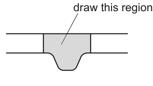
Use one ruled label line and label to identify the cuticle.
Answer
A large plan diagram of the midrib region of the leaf, occupying most of the available space, showing the following features as tissue regions (no individual cells drawn, continuous lines only, no shading):
- A thin outer line on the upper surface and a thin outer line on the lower surface representing the cuticle.
- A single line just inside each cuticle representing the upper epidermis and lower epidermis.
- A region of palisade mesophyll below the upper epidermis (drawn as a band of short, vertical lines representing the columns of cells as a tissue block).
- A region of spongy mesophyll (drawn as an irregular, loosely packed region) above the lower epidermis.
- A central vascular bundle that bulges downward into the spongy mesophyll, drawn with the correct proportions for the midrib and subdivided into:
- Xylem as the larger-celled region (drawn uppermost in the bundle)
- Phloem as the smaller-celled region (drawn below the xylem)
One ruled label line ending precisely on the cuticle, labelled cuticle.
Plan diagram of the leaf midrib with cuticle labelled, showing at least three tissues in correct proportions and a vascular bundle subdivided into xylem and phloem.
Background Concept
A plan diagram is a low-magnification outline drawing of a specimen. It shows the distribution of tissues as solid regions, NOT individual cells. The conventions of a plan diagram are:
- Lines are continuous, thin and sharp (no feathery or sketchy lines).
- No shading and no individual cells are drawn inside the tissues.
- The relative proportions of the tissues must match the specimen.
- Tissues that are subdivided (e.g. xylem and phloem inside a vascular bundle) must be shown as separate regions.
- Labels are connected with a ruled label line (drawn with a ruler) ending exactly on the structure and the name written neatly at the other end.
A typical dicotyledonous leaf, in transverse section, has the following layers from top to bottom:
- Cuticle – a waxy, waterproof layer secreted by the epidermal cells; appears as a thin outer line on both surfaces.
- Upper epidermis – a single layer of cells; in a plan diagram it is a single line.
- Palisade mesophyll – tightly packed, column-shaped cells containing many chloroplasts; drawn as a band of vertical strokes to indicate the columnar tissue.
- Spongy mesophyll – loosely packed cells with large air spaces; drawn as an irregular region.
- Vascular bundle – contains xylem (water-transporting tissue, larger cells) above and phloem (food-transporting tissue, smaller cells) below.
- Lower epidermis – single layer of cells; a single line.
- Cuticle – thin outer line on the lower surface.
The midrib is the central, thickest region of the leaf containing the main (largest) vascular bundle. Because the midrib bulges downward, the lower epidermis often dips into a V-shape beneath the vascular tissue, while the upper surface remains relatively flat.
Understanding the Question
The shaded region in Fig. 2.1 marks the midrib of a leaf transverse section (slide N1). The candidate must produce a plan diagram of ONLY this midrib region, draw it large enough to fill most of the space, and label the cuticle with a single ruled label line. The diagram must show at least three tissues and the vascular bundle must be subdivided.
Approach
- Observe the midrib on slide N1 at low power.
- Identify each tissue layer and where the vascular bundle is.
- Sketch the outline of the upper and lower surfaces, including the downward bulge of the lower epidermis at the midrib.
- Mark the inner boundaries between epidermis, palisade, spongy mesophyll, xylem and phloem.
- Draw the final plan diagram with continuous, sharp lines, no shading, no individual cells.
- Add a single ruled label line that ends on the cuticle (the outermost thin line on either surface) and write cuticle.
Step-by-Step Reasoning
- Use of space and tissue number (mark 1): The diagram must be large (filling most of the available space) and at least three different tissues must be visible. In practice, a midrib plan will usually show all of: cuticle, epidermis, palisade, spongy mesophyll, vascular bundle (xylem and phloem) — well over three tissues, which guarantees the mark.
- No cells, correct region (mark 2): Individual cells are not drawn. Only the outline of the midrib and the boundaries between tissue regions are shown. The shape of the lower surface should dip downward at the midrib because the vascular bundle is large in the midrib.
- Correct proportions of vascular tissue (mark 3): The vascular bundle in the midrib is much larger than in the rest of the leaf. Its width should be drawn in proportion to the rest of the leaf — i.e. the bundle is a substantial feature, not a tiny one.
- Subdivision of vascular tissue (mark 4): The vascular bundle is split into xylem (drawn as the larger region) and phloem (drawn as the smaller region). In a typical dicot midrib, the xylem is on the upper side and the phloem on the lower side.
- Cuticle label (mark 5): A single ruled label line must end on the cuticle (the outermost thin line on the upper or lower surface). The label is written as the word "cuticle".
Key Takeaways
- A plan diagram is a low-power outline of tissues, never of cells.
- Correct proportions and tissue subdivisions are critical for credit.
- Always use a ruled label line that ends exactly on the structure being labelled.
Common Mistakes
- Drawing individual cells inside tissues — this turns a plan diagram into a high-power drawing and loses marks.
- Forgetting to subdivide the vascular bundle into xylem and phloem.
- Label line not ending on the cuticle, or labelling the wrong structure (e.g. epidermis instead of cuticle).
- Drawing the lower epidermis as a flat line in the midrib region — it should dip down because the midrib is the thickest part of the leaf.
Things to Be Careful About
- Use a sharp pencil and a ruler for label lines.
- Keep lines continuous — no gaps or feathery strokes.
- The diagram must show the midrib region only as defined by the shaded area in Fig. 2.1, not the whole leaf.
Observe the cells in the lower epidermis surrounding the midrib on the section of the leaf on N1.
Select a line of four adjacent lower epidermal cells.
- Make a large drawing of this line of four cells.
- Use one ruled label line and label to identify the cell wall of one cell.
Answer
A large drawing of four adjacent lower epidermal cells from the lower epidermis surrounding the midrib, showing:
- Each cell drawn with two parallel lines for the cell wall (a double line, not a single thick line).
- Cells drawn as irregular, polygonal/brick-shaped (typical lower-epidermal cell shape), with the cells touching their neighbours along shared walls.
- Lines continuous, thin and sharp; no shading anywhere.
- The line of four cells drawn large enough to fill most of the available space.
- One ruled label line ending on the wall of one cell, labelled cell wall.
Large drawing of four adjacent lower epidermal cells with one cell wall labelled.
Background Concept
A high-power drawing of cells (also called a biological drawing) is drawn at high magnification using a microscope. The conventions are:
- Lines are continuous, thin and sharp — no sketchy or feathery lines.
- No shading is used; only line drawings.
- Cell walls are drawn as two parallel lines (a double line) — this represents the cellulose wall, not a single thick stroke.
- Only structures that are actually visible in the field of view are drawn; nothing is invented.
- The relative sizes and shapes of the cells must match the specimen.
- Labels are connected with a ruled label line ending exactly on the structure being named.
Lower epidermal cells of a typical dicot leaf are irregularly polygonal, often described as "brick-shaped" or jigsaw-like, and are tightly packed with no intercellular air spaces (unlike spongy mesophyll cells).
Understanding the Question
The candidate has already drawn the plan diagram of the midrib. Now they must look at the lower epidermis of slide N1 (the same slide) at higher magnification, select a line of four adjacent lower epidermal cells surrounding the midrib, and draw them as a biological (high-power) drawing. One cell wall must be labelled.
Approach
- Move the slide so the lower epidermis near the midrib is centred in the field of view.
- Increase magnification if necessary so the cell walls are clearly visible.
- Select a line of four cells that are clearly adjacent (sharing walls) and look typical of lower epidermis.
- Draw the outline of the four cells, with each cell wall as a double line.
- Use a ruler to draw one label line ending on a cell wall, and write cell wall at the other end.
Step-by-Step Reasoning
- Lines and no shading (mark 1): All lines must be continuous, thin, sharp and drawn without lifting the pencil. No hatching, stippling or coloured shading is allowed.
- Four cells touching (mark 2): Exactly four cells in a line, and each cell must share at least one wall with its neighbour. The four cells should be drawn touching, not spaced apart.
- Double cell wall (mark 3): Each cell wall is drawn as TWO parallel lines, not one thick line. This is the most frequently lost mark in cell drawings.
- Correct shape (mark 4): Lower epidermal cells are irregular, polygonal/brick-shaped (not circular, not perfectly rectangular). The shape drawn should resemble the cells in the field of view.
- Label (mark 5): A single ruled label line ending precisely on a cell wall, labelled cell wall.
Key Takeaways
- Cell walls are always drawn as two lines.
- Never shade a biological drawing.
- Always draw what you can actually see, at the correct relative size.
- Use a ruler for every label line.
Common Mistakes
- Drawing the cell wall as a single thick line (loses the mark for double wall).
- Shading inside the cells.
- Drawing the cells as perfect rectangles or perfect circles instead of their actual irregular shape.
- Drawing fewer than four cells, or four cells that don't touch each other.
- Label line not ending on the cell wall, or labelling the cytoplasm / nucleus / membrane instead of the cell wall.
Things to Be Careful About
- The lower epidermis cells do NOT contain chloroplasts (unlike palisade cells), so do not draw chloroplasts inside them.
- The four cells must be a real line of cells visible on the slide, not invented cells.
Fig. 2.2 shows a photomicrograph of a stage micrometer scale that is being used to calibrate an eyepiece graticule.
One division, on either the stage micrometer scale or the eyepiece graticule, is the distance between two adjacent lines.
The length of one division on the stage micrometer in Fig. 2.2 is .
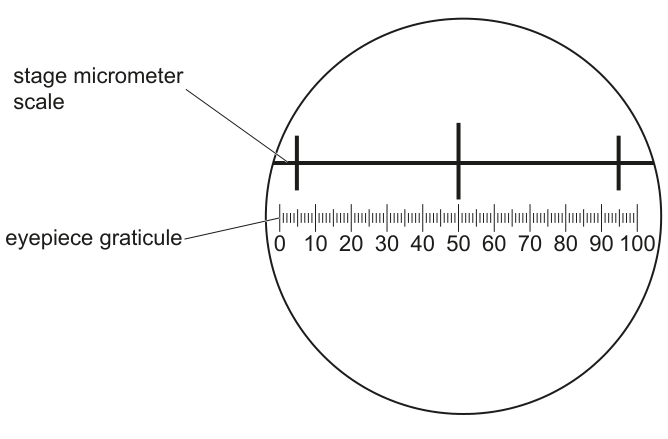
Calculate the actual length of one eyepiece graticule unit shown in Fig. 2.2.
Give your answer in micrometres ().
Show your working.
actual length = ______
Working
From Fig. 2.2, the stage micrometer shows that 1.0 mm of the stage micrometer scale corresponds to 45 eyepiece graticule divisions.
Therefore:
Answer
actual length = 22 µm (or 22.2 µm to 3 significant figures)
22 µm (or 22.2 µm)
Background Concept
An eyepiece graticule is a small glass disc with a scale etched onto it that sits inside the eyepiece of a microscope. The divisions on the graticule have NO fixed size — the actual length they represent depends on the magnification of the objective lens in use. To find out what each graticule division actually measures, the eyepiece graticule must be calibrated against a stage micrometer, which is a slide with a scale of known dimensions (here, 1.0 mm per large division, with each large division subdivided into smaller units).
Understanding the Question
Fig. 2.2 shows both scales superimposed in the field of view. The candidate must read off how many eyepiece graticule units correspond to a known length (1.0 mm) on the stage micrometer, and then convert that to micrometres (µm), since the question asks for the answer in µm.
The mark scheme awards marks for:
- Stating the correct number of eyepiece graticule units that equal 1.0 mm (45 units).
- Showing the division of 1000 µm by 45 to obtain the length of one unit in µm.
Approach
- Read the alignment: 1.0 mm on the stage micrometer = 45 divisions on the eyepiece graticule.
- Convert 1.0 mm to µm: 1 mm = 1000 µm.
- Divide 1000 by 45 to find the length of one graticule division in µm.
Step-by-Step Reasoning
- The stage micrometer scale is calibrated: 1.0 mm per large division. In Fig. 2.2 the two large marks of the stage micrometer (each separated by 1.0 mm) coincide with the 0 and 45 marks of the eyepiece graticule. So 1.0 mm = 45 eyepiece graticule divisions.
- Convert: 1.0 mm = 1000 µm.
- Therefore, 1 eyepiece graticule unit = 1000/45 µm = 22.22… µm.
- Rounded appropriately, this is 22 µm (2 sig figs) or 22.2 µm (3 sig figs). Either is acceptable for full marks.
Key Takeaways
- Always calibrate the eyepiece graticule against a stage micrometer before using it to measure specimens.
- Remember the conversion: 1 mm = 1000 µm.
- Read off the calibration carefully — errors in counting the graticule divisions are common.
Common Mistakes
- Counting the wrong number of graticule divisions (e.g. reading 50 or 40 instead of 45).
- Dividing 1.0 by 45 without converting mm to µm first (gives 0.022, then forgetting to convert units).
- Quoting the answer in mm instead of µm.
Things to Be Careful About
- The question asks for the answer in µm, so the final unit MUST be µm.
- Show the substitution clearly: 1000 ÷ 45 — this is the marking point the examiner is looking for.
- Give the answer to a sensible number of significant figures (2 or 3, matching the precision of the calibration).
Fig. 2.3 is a photomicrograph of a transverse section of a leaf from another plant of the same species as N1.
Fig. 2.3 was taken with the same microscope and the same lenses used to take the photomicrograph in Fig. 2.2.
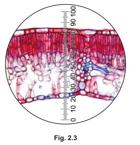
Use the calibration of the eyepiece graticule unit from (b)(i) to calculate the actual width of the leaf in Fig. 2.3.
Show your working.
actual width = ______
Working
From Fig. 2.3, the leaf section spans approximately 75 eyepiece graticule divisions (from the lower epidermis at about the 15 mark to the upper epidermis at about the 90 mark).
Using the calibration from (b)(i), 1 eyepiece graticule unit = 1000/45 µm.
Answer
actual width ≈ 1700 µm (or 1.7 mm)
1700 µm (≈ 1.7 mm)
Background Concept
Once the eyepiece graticule is calibrated (so that each division has a known actual length), the actual size of any structure can be measured by counting the number of graticule divisions it spans and multiplying by the calibration. Because Fig. 2.2 and Fig. 2.3 were taken with the same microscope and same lenses, the calibration from (b)(i) applies to Fig. 2.3 directly.
Understanding the Question
Fig. 2.3 is a photomicrograph of a leaf transverse section with the eyepiece graticule scale (0–100) superimposed vertically across the leaf. The candidate must:
- Count how many graticule divisions span the width (from upper epidermis to lower epidermis) of the leaf.
- Multiply that number by the calibration from (b)(i) (1 unit = 1000/45 µm) to obtain the actual width in µm.
Approach
- Identify the upper epidermis (top of the leaf section) and the lower epidermis (bottom of the leaf section) in Fig. 2.3.
- Read the graticule value at each surface.
- Subtract to find the number of graticule units the leaf spans.
- Multiply by the calibration (1000/45 µm per unit) and quote the answer in µm.
Step-by-Step Reasoning
- In Fig. 2.3 the upper epidermis sits at approximately the 90 mark and the lower epidermis at approximately the 15 mark on the graticule.
- Number of graticule divisions spanned = 90 − 15 = 75 divisions.
- Calibration from (b)(i): 1 division = 1000/45 µm = 22.2 µm.
- Actual width = 75 × (1000/45) µm = 75000/45 µm ≈ 1667 µm.
- This is equivalent to about 1.7 mm. Either unit is acceptable provided it is stated clearly.
Key Takeaways
- The same calibration applies whenever the same microscope and lens combination is used.
- Always read the graticule at the OUTER edges of the structure (here, the outer edges of the upper and lower epidermis).
- The marks reward stating both the graticule reading AND showing the multiplication, so write both down clearly.
Common Mistakes
- Reading the graticule at the palisade layer instead of the epidermis.
- Forgetting to multiply by the calibration (just quoting the graticule number alone).
- Quoting the answer without units, or in the wrong units.
Things to Be Careful About
- The candidate's own reading of the graticule may differ slightly from 75. The mark scheme accepts an answer that uses the student's own graticule reading multiplied by the calibration from (b)(i) — so error carried forward (ecf) is allowed: if the calibration in (b)(i) was miscalculated, the same error is accepted here as long as the method is correct.
- Give the final answer with the unit (µm) clearly stated.
Identify three observable differences, other than colour, between the leaf section on N1 and the leaf section in Fig. 2.3.
Record these three observable differences in Table 2.1.
Table 2.1
| feature | N1 | Fig. 2.3 |
|---|---|---|
Answer
| feature | N1 | Fig. 2.3 |
|---|---|---|
| thickness of the palisade mesophyll layer | thin | thick |
| number of chloroplasts visible (in palisade cells) | low / few | high / many |
| size of the vascular bundles (relative to leaf width) | large | small |
| number of vascular bundles | more | fewer |
(Any three of the above rows are sufficient for full marks.)
Three observable differences (excluding colour) include: (1) palisade layer thin in N1 vs thick in Fig. 2.3; (2) few chloroplasts in N1 vs many in Fig. 2.3; (3) vascular bundles large (N1) vs small (Fig. 2.3) relative to leaf width; (4) more vascular bundles in N1 vs fewer in Fig. 2.3.
Background Concept
When comparing two microscope specimens, only observable features should be listed — things that can actually be seen in the image. Avoid making inferences about WHY the differences exist or about the function/identity of the specimen, because the mark scheme only credits observations.
For two leaf sections of the same species (as stated in the question), the differences must be about relative proportions, thicknesses, sizes or counts of features that are directly visible — not about colour (which is explicitly excluded) and not about physiology (e.g. "higher photosynthetic rate").
Understanding the Question
The candidate has slide N1 (a leaf section they can view directly) and Fig. 2.3 (a printed photomicrograph of another leaf of the same species, taken with the same microscope). The task is to identify three observable differences between them, other than colour, and record them in the given table.
Approach
- Look carefully at N1 under the microscope (or recall the image given in the question paper) and at Fig. 2.3.
- Identify features that visibly differ between the two: thickness of layers, number of chloroplasts, size and number of vascular bundles, etc.
- Ensure each difference is observable (visible) — not an inference about function or environment.
- Write one observable difference per row of the table, with N1 in the left column and Fig. 2.3 in the right column.
Step-by-Step Reasoning
The mark scheme credits the following observable differences:
- Palisade layer thickness: In N1 the palisade layer is thin (only one or two rows of cells, or a narrow band), whereas in Fig. 2.3 the palisade layer is thick (multiple rows or a much broader band of cells).
- Number of chloroplasts: N1 shows few chloroplasts in the palisade cells, while Fig. 2.3 shows many chloroplasts (the cells in Fig. 2.3 are densely pigmented, indicating abundant chloroplasts).
- Vascular bundle size (relative to leaf width): In N1 the vascular bundles are large in proportion to the leaf width, while in Fig. 2.3 the vascular bundles are small in proportion.
- Number of vascular bundles: N1 has more vascular bundles in the field of view; Fig. 2.3 has fewer.
Any three of these four differences earn full marks (4 marks = 3 differences × at least 1 mark each, with the fourth mark often coming from completing the table correctly). The mark scheme requires that the differences be observable features — vague statements such as "N1 is healthier" or "Fig. 2.3 is from a sun leaf" do NOT earn marks.
Key Takeaways
- Always give an observable feature — something you can literally see.
- Describe the difference in both columns (N1 vs Fig. 2.3), not just one side.
- Avoid inferences about function, adaptation or environment.
- Exclude colour (as instructed).
Common Mistakes
- Stating an inference (e.g. "N1 is from a shade plant") rather than an observable feature.
- Only describing one side of the comparison (e.g. only describing N1, leaving Fig. 2.3 blank).
- Including colour as a difference (explicitly excluded by the question).
- Vague statements such as "different layers" or "different sizes" without specifying which feature and how it differs.
Things to Be Careful About
- The differences must be observable WITHOUT additional staining or physiology. Sticking to size, proportion, count, thickness, and density of visible structures is safest.
- Make sure each row in the table is filled in completely — both the feature and the descriptions of each specimen.