Biology 9700/31 — October/November 2024
Cambridge AS Level · Advanced Practical Skills · worked solutions for every part, with the mark scheme
Topics Manipulation, Measurement and Observation · Presentation of Data and Observations · Analysis, Conclusions and Evaluation · Use of the Light Microscope
Milk is sometimes contaminated with substances such as starch.
You will determine the concentration of starch in a sample of contaminated milk, using a range of starch standards.
You are provided with the materials shown in Table 1.1.
Table 1.1
| labelled | contents | hazard | volume / |
|---|---|---|---|
| M | milk | none | 50 |
| SM | 1.0% starch solution in milk (starch-milk) | none | 20 |
| CM | contaminated milk | none | 20 |
| iodine | iodine solution | irritant | 20 |
If any solution comes into contact with your skin, wash off immediately with cold water.
It is recommended that you wear suitable eye protection.
You will need to carry out a serial dilution of the 1.0% starch-milk solution, SM, to reduce the concentration by one fifth between each successive dilution.
You will need to prepare four concentrations of starch-milk solution in addition to the 1.0% starch-milk solution, SM.
You must use the milk, M, to dilute the starch-milk solution. Do not use water for the dilution.
After the serial dilution is completed, you will need to have of each concentration available to use.
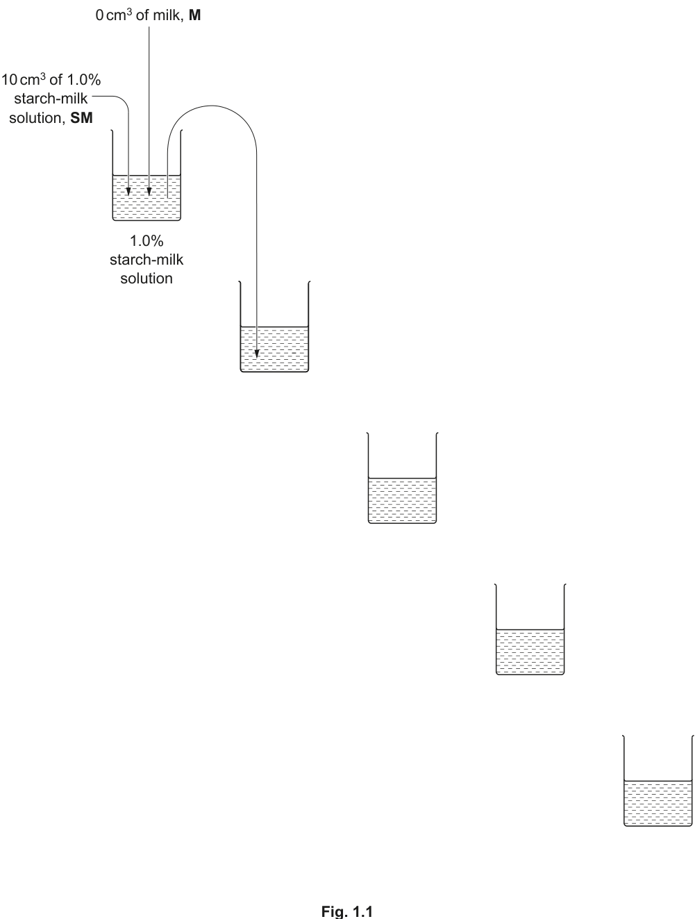
Complete Fig. 1.1 to show how you will prepare your serial dilution.
Each beaker should have:
- a labelled arrow to show the volume of starch-milk, SM, solution transferred
- a labelled arrow to show the volume of milk, M, added
- a label under the beaker to show the concentration of the starch-milk solution.
Answer
Each successive beaker contains:
| beaker | SM transferred / cm³ | M added / cm³ | concentration under beaker |
|---|---|---|---|
| 1 | — | 0 | 1.0% |
| 2 | 2 | 8 | 0.2% |
| 3 | 2 | 8 | 0.04% |
| 4 | 2 | 8 | 0.008% |
| 5 | 2 | 8 | 0.0016% |
0.2%, 0.04%, 0.008%, 0.0016% with 2 cm³ transferred and 8 cm³ of milk added at each step
Background Concept
A serial dilution is a stepwise dilution of a stock solution in which the concentration is reduced by a fixed factor at each step. Here, the dilution factor between successive beakers is 1/5 (i.e. the concentration falls to one-fifth each time).
The general rule for a 1-into-(n+1) dilution is:
- Transfer a fixed volume V of the previous (more concentrated) solution into a new container.
- Add n × V of diluent to make the total volume (n+1) × V.
- The new concentration is the previous concentration ÷ (n+1).
If the stock is 1.0% and the dilution is 1/5, the new concentrations are:
For a 1/5 dilution, a convenient choice is to transfer 2 cm³ and add 8 cm³ of diluent (milk, M, in this case), giving 2 + 8 = 10 cm³ total in each beaker. Each beaker therefore contains 8 cm³ + 2 cm³ = 10 cm³.
Understanding the Question
The question shows a partially completed Fig. 1.1: beaker 1 already contains 10 cm³ of 1.0% SM with the labels for SM and M volumes given, and a transfer arrow leads from beaker 1 to beaker 2. The candidate must complete the diagram for beakers 2–5 by adding:
- A labelled arrow into each beaker showing the volume of SM transferred from the previous beaker (2 cm³).
- A labelled arrow into each beaker showing the volume of M added (8 cm³).
- A label under each beaker stating the resulting starch-milk concentration.
The required final volume per beaker is 8 cm³ of each concentration so that 1 cm³ can be tested in step 3; this means 2 cm³ must be transferred and 8 cm³ of milk added at each stage (and the 2 cm³ taken from beaker 1 leaves 8 cm³ remaining, of which 2 cm³ is again transferred, and so on).
Approach
The strategy is to:
- Compute the four new concentrations by repeatedly dividing by 5.
- Decide a transfer/addition volume pair that gives 8 cm³ available after transfer — 2 cm³ transferred into 8 cm³ milk (total 10 cm³, 2 cm³ removed at next step leaves 8 cm³ available).
- Draw two labelled arrows into each of beakers 2–5: one for the 2 cm³ of SM coming from the previous beaker, one for the 8 cm³ of M being added, and write the concentration under each beaker.
Step-by-Step Reasoning
Step 1 — Confirm the dilution factor. The stem states "reduce the concentration by one fifth between each successive dilution", so each concentration = previous ÷ 5.
Step 2 — Compute the four new concentrations.
- Beaker 2: 1.0 / 5 = 0.2%
- Beaker 3: 0.2 / 5 = 0.04%
- Beaker 4: 0.04 / 5 = 0.008%
- Beaker 5: 0.008 / 5 = 0.0016%
Step 3 — Confirm the transfer volumes. Each beaker must end up with 8 cm³ available for use. After step 3, 1 cm³ of the standard is used, so 9 cm³ must be present before this; but more importantly the constraint is the dilution ratio: 1 part SM to 4 parts M = 2 cm³ SM + 8 cm³ M = 10 cm³. From this 10 cm³, 2 cm³ is taken into the next beaker, leaving 8 cm³ in the current beaker for use. So 2 cm³ of SM transferred + 8 cm³ of M added is the correct combination.
Step 4 — Draw the diagram. In each of the four empty beakers, add a downward arrow labelled "2 cm³ of starch-milk solution, SM" showing the transfer from the previous beaker, and a second downward arrow labelled "8 cm³ of milk, M" showing the milk being added. Under each beaker, write the appropriate concentration.
Key Takeaways
- A serial dilution requires the same dilution factor at every step, calculated as (transfer volume) / (total volume after transfer).
- For a 1/5 dilution with 10 cm³ total, the convenient pairing is 2 cm³ transferred + 8 cm³ diluent.
- The four concentrations obtained from a 1.0% stock diluted 1/5 four times are 0.2%, 0.04%, 0.008% and 0.0016%.
Common Mistakes
- Using 1 cm³ + 4 cm³ instead of 2 cm³ + 8 cm³ (still 1/5, but the volume available is too small for the procedure to be carried out on).
- Writing the concentration incorrectly because the previous concentration was used instead of dividing again (e.g. listing 0.2%, 0.02%, 0.002%, 0.0002% — this would be a 1/10 dilution, not 1/5).
- Forgetting to label the transfer arrow from the previous beaker — the mark scheme requires both arrows and the concentration label.
- Drawing water (W) into the diagram — the stem explicitly says to use milk, M, to dilute.
Things to Be Careful About
- All four concentrations must be written and must be 1/5 of the previous one.
- Both arrows into each beaker must be clearly labelled with the correct volume.
- The mark scheme requires the diagram to show 2 cm³ transferred and 8 cm³ of milk added; deviation from these exact volumes is unlikely to score if the resulting available volume is wrong.
Carry out step 1 to step 11.
step 1 Prepare the concentrations of starch-milk solution as shown in Fig. 1.1.
step 2 Label test-tubes with the concentrations prepared in step 1.
step 3 Put of the 1.0% starch-milk solution into the appropriately labelled test-tube.
step 4 Repeat step 3 with the remaining concentrations of starch-milk solution.
step 5 Add of iodine solution to each test-tube. Shake gently to mix.
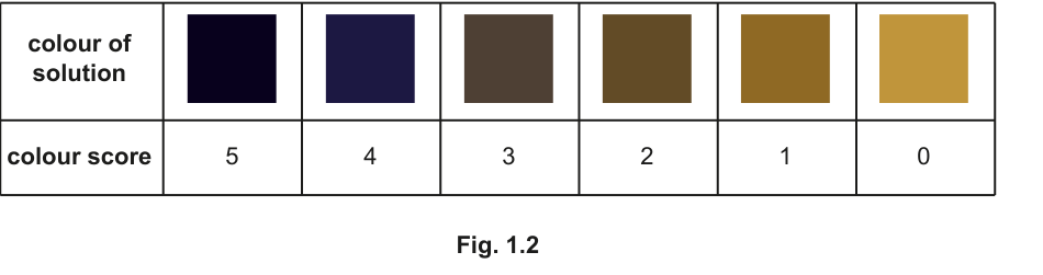
step 6 Observe the colour in each test-tube and use the key in Fig. 1.2 to determine the colour score.
step 7 Record in (a)(ii) the colour score for each concentration of starch-milk solution.
Record your results in an appropriate table.
Answer
Results table (representative — the candidate's actual colour scores will depend on the solutions tested):
| % concentration of starch-milk | colour score (0–5) |
|---|---|
| 1.0 | 5 |
| 0.2 | 4 |
| 0.04 | 3 |
| 0.008 | 1 |
| 0.0016 | 0 |
The colour score increases as the concentration of starch-milk increases: the 1.0% solution gives the highest (darkest) colour score and the 0.0016% solution gives the lowest (lightest) colour score.
Table with 'concentration of starch-milk / %' and 'colour score' headings, a recorded score for each of the five concentrations, and the correct trend (higher concentration → higher colour score).
Background Concept
Iodine forms a dark blue-black complex with starch. The intensity of this colour is proportional to the amount of starch present, so a series of starch standards of known concentration can be used to estimate the starch content of an unknown solution by colour matching.
The colour key in Fig. 1.2 turns a continuous visual gradient into a discrete numerical score (0 = no starch present, 5 = very dark blue-black), which can be tabulated and compared between samples.
Understanding the Question
After preparing the dilution series in (a)(i) and adding 1 cm³ of each to a labelled test-tube followed by 1 cm³ of iodine (step 5), the candidate observes the colour of each tube and assigns a colour score from the Fig. 1.2 key (step 6). The results must be recorded in a properly formatted table in (a)(ii).
Approach
The table needs two columns: one for the independent variable (concentration of starch-milk) and one for the dependent variable (colour score). The candidate then matches each tube to the closest swatch in Fig. 1.2 and writes the corresponding number in the table.
Step-by-Step Reasoning
Step 1 — Identify the IV and DV.
- IV: percentage concentration of starch-milk (set in (a)(i)).
- DV: colour score (0–5) read from Fig. 1.2.
Step 2 — Set up the table.
- Headings must include a quantity and (where appropriate) a unit. Here the IV heading is "% concentration of starch-milk" (the % is the unit) and the DV heading is "colour score".
- A ruled table with a column for each variable.
Step 3 — Record the colour score for each concentration. The 1.0% tube should be the darkest and so receive the highest score; as the concentration decreases, less starch is present and the iodine stays closer to its own yellow-brown colour, so the score falls towards 0.
Step 4 — State the trend. Higher concentration of starch-milk → higher (darker) colour score; the trend should be a clear positive relationship across the five concentrations, with the 1.0% tube darker than the 0.0016% tube.
Key Takeaways
- A results table must have clear headings giving both the quantity and the unit for each column.
- A colour key turns a qualitative observation into a numerical score so the results can be tabulated and compared.
- The expected relationship is positive: more starch produces a darker blue-black colour with iodine, hence a higher score on the key.
Common Mistakes
- Omitting the unit in the heading (e.g. just writing "concentration" rather than "% concentration of starch-milk").
- Recording colours as descriptions ("dark blue", "light brown") rather than the numerical score from the key.
- Inverting the trend (writing the highest concentration with the lowest score).
- Leaving rows blank — every concentration prepared in (a)(i) must have a recorded score.
Things to Be Careful About
- The trend is described by the mark scheme as "the colour score for 1% starch-milk is higher than the colour score at the lowest concentration of starch-milk" — both ends of the range should be referenced, not just a vague "colour score decreases as concentration decreases".
To determine the concentration of starch in the contaminated milk, CM, you will need to test a sample of CM.
State the volume of CM that you will use.
volume = ______
Answer
volume = 1 cm³
1
Background Concept
In any colorimetric comparison, the volume of sample tested must match the volume used for the standards exactly, otherwise the amount of colour produced (and therefore the apparent score) will not be comparable.
Understanding the Question
Step 3 instructs the candidate to "put 1 cm³ of the 1.0% starch-milk solution into the appropriately labelled test-tube". To compare the colour of the contaminated milk (CM) with the standards, the same volume of CM must be used in step 9.
Approach
Simply repeat the volume used in step 3, since the colour comparison relies on having the same total volume of test liquid and the same volume of iodine in every tube.
Step-by-Step Reasoning
The standards each received 1 cm³ of starch-milk + 1 cm³ of iodine. For CM, exactly 1 cm³ of CM + 1 cm³ of iodine must be used so the colour intensities are directly comparable with the standards in the colour key.
Key Takeaways
- A colorimetric comparison requires the test sample and the standards to be measured in equal volumes, with equal volumes of reagent added.
Common Mistakes
- Choosing a different volume (e.g. 2 cm³) "to make the colour more visible" — this would change the intensity and make the result uncomparable with the standards.
Things to Be Careful About
- State the unit (cm³) clearly; the answer must be a number with the unit shown.
step 8 Label a test-tube CM.
step 9 Transfer the volume of CM that you stated in (a)(iii) into test-tube CM.
step 10 Put of iodine solution into the test-tube. Shake gently to mix.
step 11 Observe the colour in the test-tube, and use the key in Fig. 1.2 to determine the colour score.
Record the colour score for test-tube CM.
colour score for CM = ______
Answer
colour score for CM = (a whole number 0–5 read from Fig. 1.2; representative value, e.g. 3, with 1 cm³ CM + 1 cm³ iodine producing a mid-brown colour)
The exact value depends on the candidate's CM sample; write the score (0, 1, 2, 3, 4 or 5) that most closely matches the colour of the CM + iodine tube against the Fig. 1.2 swatches.
A whole number between 0 and 5 (e.g. 3), read from Fig. 1.2.
Background Concept
The same iodine–starch chemistry applies here: the more starch in the contaminated milk, the more blue-black complex forms, and the higher the score on the Fig. 1.2 key.
Understanding the Question
In step 11 the candidate compares the colour of the CM + iodine tube with the swatches in Fig. 1.2 and records the corresponding number (0 = palest yellow-brown, 5 = darkest blue-black). The value is a single integer.
Approach
Hold the CM tube next to the Fig. 1.2 chart under the same lighting and pick the swatch that most closely matches. Write the score on the answer line.
Step-by-Step Reasoning
Because the result is student-dependent, the only mark-scheme requirement is that a valid score (0–5) is recorded. The scoring convention is identical to that used in (a)(ii), so the same reading technique applies.
Key Takeaways
- Reading a colour score requires a direct side-by-side comparison under consistent lighting.
- The result must be a single integer; "between 2 and 3" or "darkish brown" is not a valid answer.
Common Mistakes
- Writing a non-integer or a description ("brown-ish") rather than the score.
- Comparing the colour after the iodine has begun to settle, which can give a misleading lighter appearance.
Things to Be Careful About
- The score should be read immediately after mixing, before any settling of the colour.
Use your results in (a)(ii) and (a)(iv) to determine the concentration of starch in the contaminated milk, CM.
concentration of starch in CM = ______
Answer
concentration of starch in CM = (the % concentration of the starch-milk standard whose colour score in (a)(ii) matches the colour score recorded for CM in (a)(iv); if the score lies between two standards, give a value between the two concentrations, e.g. between 0.008% and 0.04%)
A worked example: if the CM tube gave a colour score of 3, the concentration of starch in CM is 0.04% (since 0.04% gave a score of 3 in the table above).
The starch-milk concentration whose colour score matches the CM score (e.g. 0.04% if the CM score = 3).
Background Concept
A standard series provides known reference points; an unknown sample is quantified by finding the standard whose response (here, colour score) it most closely matches. This is the principle of colorimetric estimation.
Understanding the Question
Using the table completed in (a)(ii) and the CM score from (a)(iv), the candidate must read off (or estimate) the concentration of starch in CM that would produce that score.
Approach
Find the row in the (a)(ii) table whose colour score equals the CM score. The corresponding concentration in the first column is the answer. If the CM score lies between two standards, give a value between the two concentrations.
Step-by-Step Reasoning
- If CM score = 5 → concentration = 1.0% (or higher; the method can only estimate within the range tested).
- If CM score = 4 → concentration = 0.2%.
- If CM score = 3 → concentration = 0.04%.
- If CM score = 1 or 2 → concentration between 0.0016% and 0.008% (or 0.008% and 0.04% respectively).
- If CM score = 0 → concentration = 0.0016% or lower (below the detectable range).
The mark scheme credits any value that is consistent with the candidate's own results from (a)(ii) and (a)(iv).
Key Takeaways
- A colorimetric estimation works by matching the unknown to a standard, or by interpolating between two adjacent standards.
- The estimate is only valid within the range of the standards used; a "5" or a "0" indicates the unknown is beyond the range.
Common Mistakes
- Picking a concentration that does not match the recorded score (e.g. writing "1.0%" when the CM score is 2).
- Writing the answer without the % unit.
Things to Be Careful About
- The concentration must be quoted as a percentage to be consistent with the standards; do not invent a different unit.
Answer
The colour in the test-tubes has to be matched by eye to the swatches in Fig. 1.2, which is subjective; different observers (or the same observer on different days) may assign different scores to the same tube.
Matching the colour in the test-tube to a colour score is subjective / difficult to judge accurately.
Background Concept
A source of error in a practical is any feature of the procedure that introduces uncertainty into the result. Sources of error are distinguished from improvements: an error describes the problem, an improvement describes how it could be reduced.
Understanding the Question
Step 6 asks the candidate to compare the colour of each test-tube with the swatches in Fig. 1.2 and assign a score. The mark scheme requires the candidate to identify the difficulty of this colour-matching step as the source of error.
Approach
Think about what is uncertain in step 6. The colour comparison is done by eye, with no instrument, so the score is partly a matter of judgement.
Step-by-Step Reasoning
- The colour score is read against six discrete swatches, but the actual tube colour is continuous.
- Two observers can legitimately assign different scores to the same tube (e.g. one reads 2, the other reads 3).
- Even one observer may hesitate between two adjacent swatches, especially for tubes whose colour lies between them.
- This subjectivity introduces uncertainty into the (a)(ii) table and the (a)(v) estimate.
Key Takeaways
- Sources of error describe specific, identifiable weaknesses in the procedure; "human error" or "inaccuracy" are too vague to score.
- Where a colour change is used to score a result, the subjectivity of colour matching is the usual source of error.
Common Mistakes
- Writing "human error" or "the experiment was not accurate" — too vague to score.
- Describing an improvement (e.g. "use a colorimeter") rather than the error.
- Naming a problem with a different step (e.g. "not rinsing the test-tubes") when step 6 is the one in question.
Things to Be Careful About
- The mark scheme credits the specific point that matching the colour to a score is difficult; the answer should say so plainly.
Answer
Milk itself has a slight colour (an off-white / pale yellow). If water were used to dilute the starch-milk, it would dilute (change) this background colour of the milk, so the colour of the diluted solution after adding iodine would no longer be comparable with the contaminated milk sample being tested.
Water would dilute the colour of the milk itself, so the colours would not be comparable with CM.
Background Concept
When a coloured substance is being analysed, the matrix (everything else in the solution) contributes to the overall colour. If the matrix is altered by the diluent, the colour comparison is no longer fair. Keeping the diluent the same as the bulk of the unknown sample keeps the background matrix constant.
Understanding the Question
The unknown being tested is contaminated milk (CM), which is mostly milk. The standards are made by diluting starch-milk (SM) with plain milk (M), not water. The candidate must explain why milk is the appropriate diluent.
Approach
Compare the effect of using water vs milk on the background colour of the resulting solution. If the background changes, the iodine + starch colour is no longer the only variable.
Step-by-Step Reasoning
- Milk has a natural off-white / pale yellow colour.
- Diluting with water would lighten this background as well as dilute the starch, so the appearance of the standard tubes (after adding iodine) would be different from CM + iodine even at the same starch concentration.
- Diluting with milk keeps the background matrix (colour, opacity, suspended solids) identical to CM, so any difference between a standard tube and the CM tube is due to the starch concentration only.
- Therefore the comparison in the (a)(v) estimate is valid only because milk is the diluent.
Key Takeaways
- Standards for a colorimetric test should be prepared in the same matrix as the unknown sample, otherwise the background contributes differently to the colour.
- "Matrix-matched" standards are a basic requirement of any quantitative colour test.
Common Mistakes
- Saying "milk is safer than water" or "water would react with the milk" — neither is the reason.
- Saying "milk contains starch" — milk contains only trace amounts, not enough to affect the test.
Things to Be Careful About
- The mark scheme credits the specific idea that water would dilute the colour (of the milk matrix); an answer that simply says "so the colours are the same" without naming the matrix effect is weaker but may still score.
Milk is sometimes contaminated with glucose.
Suggest how you would modify this investigation to determine the concentration of glucose in a sample of contaminated milk.
Answer
- Replace iodine with Benedict's solution (which detects reducing sugars such as glucose) and heat the mixture to greater than 80 °C (or boil it).
- Measure the time taken for the first colour change (e.g. from blue to green/yellow/orange/red) and use that time to estimate the glucose concentration, comparing against a glucose-in-milk standard series tested in the same way.
Use Benedict's solution and heat above 80 °C; measure the time to the first colour change.
Background Concept
Iodine detects starch specifically (it forms a blue-black complex with the helical amylose molecule). Glucose is a reducing sugar and does not give a colour with iodine; it is instead detected by Benedict's (or Fehling's) reagent, which contains Cu²⁺ ions that are reduced to red Cu₂O on heating with a reducing sugar. The intensity of the final colour (and the time taken to reach it) depends on the concentration of reducing sugar present.
Understanding the Question
The original procedure uses iodine to detect starch and the depth of blue-black colour to estimate the starch concentration. The candidate must modify the procedure to estimate glucose instead. The modification must:
- Use a reagent that reacts with glucose (Benedict's solution).
- Provide a quantitative measure (the time to the first colour change), not just a final colour, so that different concentrations of glucose can be distinguished.
Approach
Replace the colour-match endpoint of the iodine test with a time-based endpoint for the Benedict's test. The faster the first colour change, the higher the glucose concentration. Compare the CM result with a glucose-in-milk standard series treated identically.
Step-by-Step Reasoning
Step 1 — Choose the reagent. Benedict's solution contains CuSO₄, Na₂CO₃ and Na citrate. On heating with a reducing sugar, the blue Cu²⁺ is reduced to a red/orange Cu₂O precipitate, producing a sequence of colours: blue → green → yellow → orange → brick-red. The colour and the time taken to reach the first change indicate the sugar concentration.
Step 2 — Specify the heating conditions. Benedict's reaction only proceeds efficiently at high temperature; the mixture must be heated to > 80 °C, and in practice the test tubes are placed in a boiling water bath.
Step 3 — Specify the quantitative measurement. A simple "observe the colour at the end" is qualitative. To make the test quantitative, the time taken for the first appearance of the new (non-blue) colour is measured with a stop-clock. A higher glucose concentration reduces Cu²⁺ more quickly, so the first colour change occurs sooner. The time is compared with a glucose-in-milk standard series (e.g. 0.1%, 0.2%, 0.4%, 0.8% glucose in milk) treated identically.
Step 4 — State the modification in the order the mark scheme requires.
- Use Benedict's solution and heat to > 80 °C / boil.
- Measure the time to the first colour change.
Key Takeaways
- Iodine detects starch; Benedict's detects reducing sugars such as glucose.
- A qualitative "yes/no" colour test can be made quantitative by timing the appearance of the colour change.
- Any quantitative test must include a standard series for comparison.
Common Mistakes
- Suggesting iodine again ("use a more concentrated iodine solution") — iodine does not react with glucose.
- Suggesting Benedict's but not mentioning heating, or saying "leave at room temperature" — the reaction will not proceed.
- Suggesting only the final colour, not a measurable end-point (e.g. "record the colour produced") — this is qualitative and does not give a number to plot against a standard series.
- Suggesting Biuret reagent (which detects peptide bonds / protein), not glucose.
Things to Be Careful About
- Both mark points are needed: the reagent AND the quantitative measurement. Stating only one of them scores only one mark.
Some people are intolerant to lactose in milk. The enzyme -galactosidase is used to break down the lactose in milk.
In an investigation, equal quantities of -galactosidase were added to different concentrations of lactose in milk. The rate of lactose breakdown was measured and recorded.
The results are shown in Table 1.2.
Table 1.2
| concentration of lactose / | rate of reaction / arbitrary units |
|---|---|
| 12 | 0.30 |
| 42 | 0.65 |
| 70 | 0.80 |
| 110 | 1.15 |
| 164 | 1.25 |
| 210 | 1.25 |
Answer
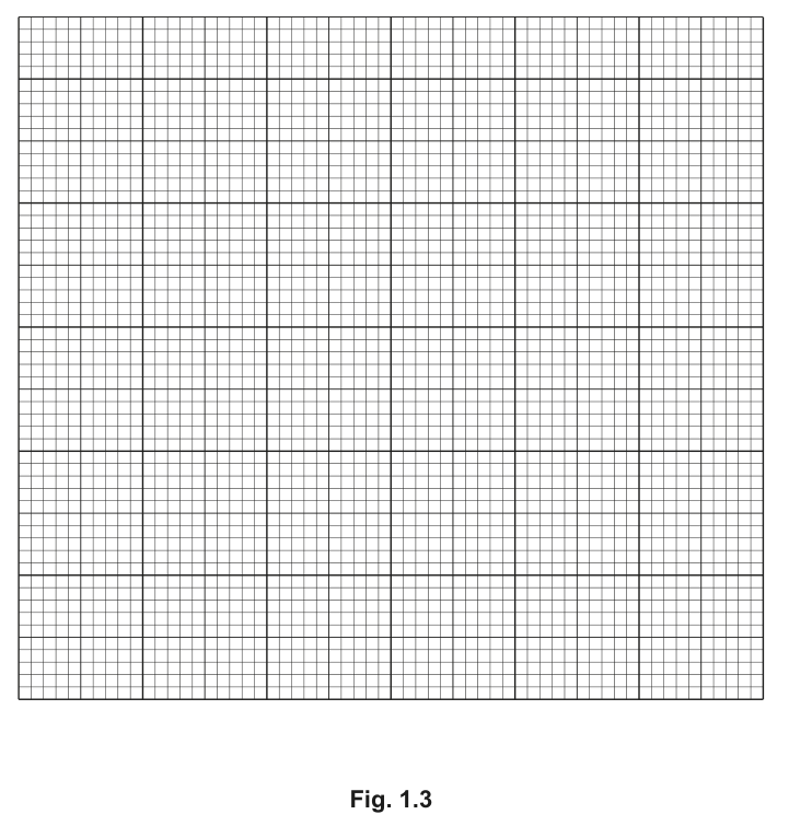
Plot the following six points on the grid in Fig. 1.3 and join them with a smooth curve:
| concentration of lactose / mmol dm⁻³ | rate of reaction / arbitrary units |
|---|---|
| 12 | 0.30 |
| 42 | 0.65 |
| 70 | 0.80 |
| 110 | 1.15 |
| 164 | 1.25 |
| 210 | 1.25 |
- x-axis: concentration of lactose / mmol dm⁻³, with a linear scale from 0 to ≥ 220 (e.g. 0, 40, 80, 120, 160, 200).
- y-axis: rate of reaction / arbitrary units, with a linear scale from 0 to ≥ 1.25 (e.g. 0, 0.25, 0.50, 0.75, 1.00, 1.25).
- Mark each point with a small cross or a dot in a circle.
- Draw a smooth, thin line through all the points (it rises steeply at first, then flattens to a plateau at 1.25).
Smooth curve through (12, 0.30), (42, 0.65), (70, 0.80), (110, 1.15), (164, 1.25), (210, 1.25), with axes labelled and linear scales.
Background Concept
A scatter graph plots two continuous variables, one on each axis, to show the relationship between them. A line of best fit (straight or curved) is drawn through the points to summarise the trend.
For enzyme-kinetics data of this type, the rate initially rises with substrate concentration but then levels off as the enzyme's active sites become saturated — the curve is therefore a hyperbola-like shape, not a straight line.
Understanding the Question
Table 1.2 gives six paired (concentration, rate) values. The candidate must plot these on the grid in Fig. 1.3 with the correct axes, scales, plotted points and a smooth curve joining them.
Approach
- Identify the IV and DV and assign them to the x- and y-axes.
- Choose a linear scale for each axis that uses at least half the grid and gives convenient labelled intervals.
- Plot each pair as a small cross (×) or a dot inside a circle (⊙).
- Join the points with a smooth curve that follows the trend — steeply rising at first, then flattening to a plateau.
Step-by-Step Reasoning
Step 1 — Axes.
- x-axis (horizontal): concentration of lactose, with units mmol dm⁻³. Range to plot: 0 to 210. A convenient scale is 0–220 in steps of 40 mmol dm⁻³ (0, 40, 80, 120, 160, 200).
- y-axis (vertical): rate of reaction, units "arbitrary units". Range to plot: 0 to 1.25. A convenient scale is 0–1.25 in steps of 0.25 (0, 0.25, 0.50, 0.75, 1.00, 1.25). The mark scheme requires the scale to be at least 0.25 to 2 cm and labelled at least every 2 cm — i.e. an interval of 0.25 per 2 cm is correct.
Step 2 — Plot the six points.
- (12, 0.30)
- (42, 0.65)
- (70, 0.80)
- (110, 1.15)
- (164, 1.25)
- (210, 1.25)
Each point should be marked with a small, neat cross or a dot in a circle, with the centre of the mark exactly on the value.
Step 3 — Draw the curve.
- The curve rises steeply between 12 and 70 mmol dm⁻³, levels off through 110 mmol dm⁻³ and is essentially flat at 1.25 from 164 to 210 mmol dm⁻³.
- Draw a single smooth, thin line that passes through (or very close to) all six points; do not join the points with a series of straight zig-zag segments.
Key Takeaways
- A graph must have labelled axes (with units), a linear scale that uses at least half the grid, accurately plotted points and an appropriate line of best fit.
- Where the relationship is non-linear (as here, with saturation), a smooth curve is drawn through the points rather than a straight line.
- "Rate" goes on the y-axis because it is the dependent variable (the quantity being measured in response to a change in substrate concentration).
Common Mistakes
- Putting concentration on the y-axis and rate on the x-axis (the IV must be on the x-axis).
- Using a non-linear or awkward scale (e.g. 12, 24, 36, 48 …) that compresses the data into a small region of the grid.
- Drawing straight line segments between every pair of points ("dot-to-dot") instead of a smooth curve.
- Forgetting the units in the axis labels (just writing "concentration of lactose" without "mmol dm⁻³").
- Drawing a line that does not pass through the points (e.g. forcing a straight line through the whole data set, which ignores the obvious plateau).
Things to Be Careful About
- The mark scheme requires each of: correct axis labels with units; suitable linear scales; correct point plotting with × or ⊙; and a smooth, thin line through all the points. Missing any one costs a mark.
- The two highest points (164 and 210) have the same y-value, so the curve is horizontal between them — this is the visual signature of saturation and must be preserved.
Answer
- The rate of reaction increases as the concentration of lactose increases, up to about 110 mmol dm⁻³, and then plateaus (levels off) at 1.25 arbitrary units between 164 and 210 mmol dm⁻³.
- Initially, increasing the substrate concentration provides more lactose molecules to bind to the active sites of β-galactosidase, so more enzyme–substrate complexes form per unit time and the rate rises.
- At higher lactose concentrations the active sites of the enzyme become saturated — all of the β-galactosidase molecules are already bound to substrate — so adding more lactose cannot increase the rate further and the curve levels off.
Rate increases with lactose concentration then plateaus; more substrate is available at first, then the active sites become saturated.
Background Concept
Enzymes are biological catalysts that speed up reactions by binding substrate molecules at their active sites. For a fixed amount of enzyme, the rate of reaction depends on how often enzyme and substrate collide productively.
- When substrate is in short supply, the active sites are mostly empty and the rate is limited by the availability of substrate.
- As substrate concentration increases, more active sites are occupied at any moment, so the rate rises.
- Once every active site is occupied (the enzyme is "saturated"), the rate cannot increase further; it is now limited by the speed at which the enzyme can convert substrate to product and release it. This is the plateau region.
This is the classic Michaelis–Menten / saturation curve, and the plateau is described by (the maximum rate).
Understanding the Question
The graph plotted in (b)(i) shows a curve that rises steeply at low lactose concentrations and then levels off at high concentrations. The candidate must (1) describe this shape and (2) explain it in terms of substrate availability and active-site saturation.
Approach
Describe the shape in two parts — what happens initially and what happens later. Then explain each part in terms of the underlying enzyme mechanism.
Step-by-Step Reasoning
Part 1 — Describe the shape.
- From 12 to ~110 mmol dm⁻³, the rate rises from 0.30 to 1.15.
- From ~110 to 210 mmol dm⁻³, the rate levels off at 1.25 (the same value at 164 and 210 mmol dm⁻³).
- So the curve is increasing and then plateauing.
Part 2 — Explain the initial rise.
- At low lactose concentrations there are not many substrate molecules available, so the active sites of the (fixed quantity of) β-galactosidase are mostly empty.
- Increasing the lactose concentration puts more substrate molecules in solution, which collide with the active sites more often, forming enzyme–substrate complexes more often, so the rate of lactose breakdown increases.
Part 3 — Explain the plateau.
- At high lactose concentrations, every active site of every β-galactosidase molecule is already occupied (the enzyme is saturated).
- The active sites cannot work any faster, so adding more substrate cannot increase the rate.
- The rate is now limited by the turnover number of the enzyme (the time taken to convert one substrate molecule to product and release it), not by substrate availability.
Key Takeaways
- A rate vs substrate concentration graph for an enzyme-catalysed reaction is a hyperbola: it rises and then plateaus.
- The rising portion is limited by substrate availability; the plateau is limited by active-site saturation ().
- "Describe and explain" requires both what the graph shows AND why — a description without the explanation scores only partial credit.
Common Mistakes
- Describing only the rise and not the plateau, or vice versa — both must be mentioned.
- Saying "the enzyme is used up" or "the enzyme is denatured" at high concentrations — denaturation is caused by high temperature / pH, not by high substrate.
- Saying "there is more enzyme at higher concentrations" — the question states equal quantities of enzyme were used, so this is wrong.
- Saying "the reaction is in equilibrium" — the question is about initial rate, not equilibrium.
Things to Be Careful About
- The mark scheme credits three points: (1) rate increases then plateaus; (2) rate increases as more substrate is available; (3) active sites become saturated. All three should appear for full marks.
J1 is a slide of a stained transverse section through a leaf.
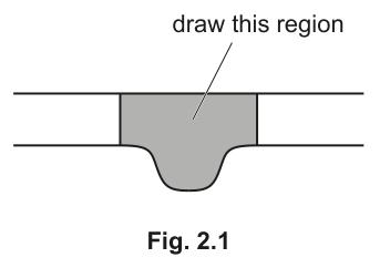
Draw a large plan diagram of the region of the leaf on J1 indicated by the shaded area in Fig. 2.1.
Use a sharp pencil.
Use one ruled label line and label to identify the lower epidermis.
Answer
A large plan diagram of the leaf region shown by the shaded area in Fig. 2.1, drawn with a sharp pencil, no shading and no individual cells.
The plan diagram must show:
- A flat upper surface drawn as a single thin continuous line (upper epidermis).
- A palisade mesophyll band immediately below the upper epidermis, drawn in the correct proportion — the palisade should occupy roughly one-quarter to one-third of the total depth of the leaf (excluding the midrib bulge).
- A spongy mesophyll region below the palisade, drawn as an irregular but continuous area.
- A central midrib that protrudes below the rest of the lower surface of the leaf, with the vascular bundle shown clearly and subdivided (xylem on the upper side, phloem on the lower side).
- The lower epidermis drawn as a single thin continuous line that follows the lower surface of the leaf, including around the protruding midrib.
- One ruled label line (no arrowhead) ending in the lower epidermis, with the text "lower epidermis" at the other end.
The drawing should occupy most of the available space and use thin, continuous lines.
Large plan diagram of the shaded leaf region: flat upper epidermis, palisade band (~1/4–1/3 of leaf depth), spongy mesophyll, protruding midrib with subdivided vascular bundle, lower epidermis following the lower contour; one ruled label line to the lower epidermis.
Background Concept
A plan diagram is a low-magnification, simplified drawing of a tissue that conveys the arrangement of tissues but deliberately omits cellular detail. It is the standard way to summarise a microscope field when the question asks for the "big picture" of a specimen.
In a typical dicotyledonous leaf transverse section, from upper to lower surface, the tissues are:
- Upper epidermis – a single layer of cells, often with a cuticle.
- Palisade mesophyll – tightly packed column-shaped cells rich in chloroplasts, just below the upper epidermis where light intensity is highest.
- Spongy mesophyll – irregularly shaped cells with large intercellular air spaces for gas exchange.
- Vascular bundle (xylem and phloem) – xylem lies on the upper side of the bundle, phloem on the lower side; both are usually enclosed in a bundle sheath.
- Lower epidermis – a single cell layer containing stomata.
The shaded area in Fig. 2.1 includes the midrib and the lamina on either side; the midrib region protrudes below the rest of the leaf, which is the most distinctive feature to capture in the plan diagram.
Understanding the Question
This is a drawing task (Paper 3 convention). The candidate must:
- Look down the microscope at slide J1 and select the field that matches the shaded area in Fig. 2.1.
- Draw a plan diagram of that field.
- Add one ruled label line and label identifying the lower epidermis.
The command word is draw, not describe — the actual drawing on the answer sheet is what earns the marks. A description in words, however accurate, would score zero.
Approach
Before touching the pencil, identify the features in the shaded region:
- A flat, roughly horizontal upper surface (upper epidermis).
- A palisade layer that is several cells deep (this is the band to estimate the depth of — it should be drawn as a thicker band, but proportionally to the rest of the leaf).
- A spongy mesophyll region with air spaces.
- A midrib that bulges below the rest of the leaf, containing a vascular bundle that should be subdivided into xylem (upper) and phloem (lower).
Then plan the drawing on paper:
- Decide where the top and bottom lines go and use most of the available space.
- Mark a guideline for the lower edge of the palisade layer.
- Mark where the midrib starts and ends on the lower surface.
- Add the subdivision of the vascular bundle.
- Add the single required label.
Step-by-Step Reasoning
-
Mark 1 – most of the available space and no shading. Draw a diagram that fills at least two-thirds of the answer space. Do not shade any region; use only outline.
-
Mark 2 – correct region and no cells. The drawing must show the midrib plus the lamina on both sides (the entire shaded area in Fig. 2.1). The drawing must contain no individual cells — outlines of tissues only. (If a candidate draws the brick-like outline of palisade cells, this is a high-power drawing, not a plan diagram, and the cell penalty applies.)
-
Mark 3 – correct proportion of palisade layer. Look at the actual slide: the palisade layer is several cells thick but the whole leaf is much thicker. The plan diagram must reflect this — a band that occupies roughly 1/4–1/3 of the total leaf depth, not a hairline and not half the leaf.
-
Mark 4 – area under the vascular bundle and subdivision of the bundle. The midrib bulges below the lower epidermis of the lamina. Inside the bundle, draw a line separating the xylem (upper part of the bundle) from the phloem (lower part). This is the only way to communicate that the candidate understood the bundle's internal structure.
-
Mark 5 – ruled label line and label to the lower epidermis. A single, straight, ruler-drawn line ends in contact with the lower epidermis. The other end terminates in the text "lower epidermis". No arrowhead, no gap, no extra labels.
Key Takeaways
- A plan diagram = tissue outlines only, no individual cells, no shading, thin continuous lines.
- Proportions matter — judge them by eye from the actual slide, not from the textbook.
- One clean label line is required; do not overload the diagram with arrows.
- A label line must end in the structure being labelled — it should not stop in the air beside it.
Common Mistakes
- Drawing individual cells (turning the plan into a high-power drawing).
- Shading any region.
- Drawing the midrib flush with the rest of the lower surface (forgetting the bulge visible in Fig. 2.1).
- Forgetting to subdivide the vascular bundle (xylem above, phloem below).
- Using arrowheads on the label line, or letting the line float beside the lower epidermis instead of touching it.
- Labelling the upper epidermis or any other structure (only the lower epidermis is required and additional labels add no credit here).
Things to Be Careful About
- Use a sharp HB (or harder) pencil and a ruler for the label line so the lines are crisp.
- Keep all outlines continuous — no breaks where the pen/pencil is lifted.
- The proportions of the palisade layer should be checked against the slide, not the textbook — what looks "right" varies between specimens.
- Do not draw cells even to "show what the palisade looks like" — that belongs in a high-power drawing, not here.
Observe the xylem vessel elements in the leaf on J1.
Select a line of four adjacent xylem vessel elements.
Each xylem vessel element must touch at least one other xylem vessel element.
- Make a large drawing of this line of four xylem vessel elements.
- Use one ruled label line and label to identify the wall of one xylem vessel element.
Answer
A large drawing of four adjacent xylem vessel elements, with each cell touching at least one other cell. The drawing must use a sharp pencil with continuous, thin and sharp lines.
Each xylem vessel element must be drawn with:
- A double-line wall (two parallel lines representing the two surfaces of the thick lignified cell wall).
- A polygonal shape with 4 or 5 sides (correct shape of xylem vessel elements, which are typically rectangular or pentagonal in cross-section).
- Where two cells touch each other, three lines must be visible between them (the inner wall of cell A, the contact region / middle lamella between the two walls, and the inner wall of cell B — together producing three parallel lines).
The four cells should occupy most of the available space, arranged in a line so that each cell touches at least one neighbour.
A single ruled label line (no arrowhead) ending at the wall of one xylem vessel element, with the text "wall" (or "cell wall") at the other end.
Drawing of four adjacent polygonal xylem vessel elements, each with a double-line wall, three lines between adjacent cells, only four cells drawn, label line to the wall of one vessel element.
Background Concept
At high magnification, biological drawings must convey the three-dimensional nature of cells. The standard CIE convention is:
- Each cell wall is drawn as two parallel lines, representing the inner and outer surfaces of the wall.
- Where two cells are adjacent, the double walls of the two cells are visible together — producing three lines between adjacent cells (inner wall of A, contact region between the two walls, inner wall of B). For xylem, the walls are thick and lignified, so the "contact region" is appreciable and the three lines are clearly separated.
Xylem vessel elements are dead, lignified cells whose end walls have broken down to form continuous vessels for water transport. In cross-section they appear as large, polygonal, thick-walled cells (usually 4–6 sides), often stained red or pink with typical stains such as safranin.
Understanding the Question
The candidate must:
- Switch to a high-power objective and locate a line of xylem vessel elements in slide J1.
- Select a contiguous row of four such elements, where each element touches at least one other (i.e. no isolated single cell).
- Draw the four cells accurately.
- Add one label: the wall of one of the cells.
The command word is again draw — the marks are awarded to the drawing on the answer sheet, not to a description.
Approach
Locate a clear row of xylem elements at high power. Pick a row where:
- The cells are clearly polygonal (4–5 sides), not crushed or distorted.
- Each cell is in clear contact with at least one neighbour.
- The walls are thick and clearly visible, so the double-line convention can be applied.
Plan the drawing so the four cells occupy most of the available space and you can show the wall convention clearly on at least one junction between cells.
Step-by-Step Reasoning
-
Mark 1 – most of the available space; lines continuous, thin and sharp. Use a sharp pencil. Each line should be drawn in one smooth stroke with no break, no feathering, and no thick line. The drawing should fill at least two-thirds of the answer space.
-
Mark 2 – only four xylem vessel elements, each touching at least one other. Count the cells in the drawing before submitting — there must be exactly four, and every cell must share a wall with at least one neighbour (so the four cells form a connected line, e.g. cell 1 – cell 2 – cell 3 – cell 4). Drawing five or more cells loses this mark.
-
Mark 3 – two lines around each vessel; three lines where cells touch. Apply the double-line wall convention: each individual cell is bounded by two parallel lines, even where the cell is on the outside of the row. Where two cells are in contact, you should see three parallel lines: inner wall of cell A — contact region between the two walls — inner wall of cell B. This must be visible at least at one cell–cell junction.
-
Mark 4 – correct shape of cells (4 or 5 sides). Xylem vessel elements in cross-section are polygonal, not round, not amorphous, and not star-shaped. Aim for cells with 4 or 5 straight sides, drawn in proportion to the microscope image.
-
Mark 5 – ruled label line to the wall of one xylem vessel element. Draw one straight, ruler-drawn line ending in contact with a cell wall. The other end terminates in the text "wall" (or "cell wall"). No arrowhead, no gap, no extra labels.
Key Takeaways
- High-power drawings of cells use the double-line wall convention to convey the 3D nature of the wall.
- Where two cells touch, you should see three lines, not one and not two.
- Only the requested number of cells is drawn — counting matters.
- The cells in xylem are polygonal (4–6 sides), not round.
- One label line only; the line must end in the structure being labelled.
Common Mistakes
- Drawing only one line per cell wall (loses the double-line mark and often the three-lines-between-cells mark).
- Drawing five or more cells, or four cells where one is not actually touching the others.
- Drawing the cells as circles or ovals instead of polygons.
- Using arrows on the label line, or letting the label line stop in the lumen of the cell (it must end on the wall, not in the open space inside the cell).
- Labelling the lumen, the cytoplasm, the nucleus, or any feature that is not the wall.
Things to Be Careful About
- Use a sharp pencil and keep lines thin so that the double-line convention is visible.
- Count the cells before submitting — exactly four is required.
- The label line must end on the wall, not in the lumen and not in the middle lamella region.
- The mark scheme accepts the label text "wall" or "cell wall" — do not write "xylem vessel" or any other wording as the label here, because the question asks specifically for the wall.
Fig. 2.2 is a photomicrograph of a transverse section through a different leaf from J1.
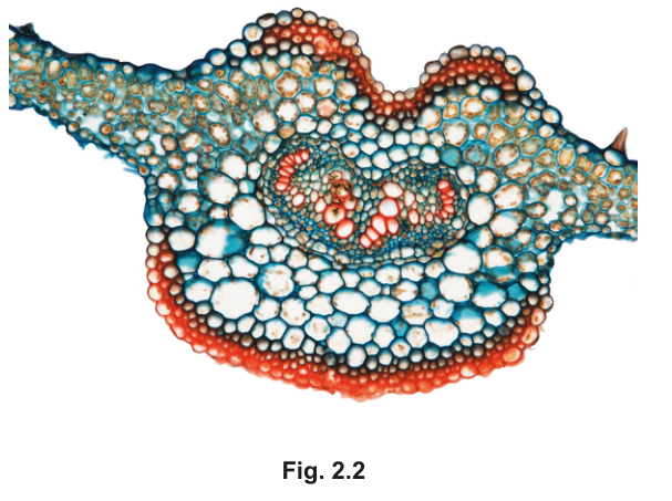
Identify three observable differences, other than colour, between the section on J1 and the section in Fig. 2.2.
Record these three observable differences in Table 2.1.
Table 2.1
| feature | J1 | Fig. 2.2 |
|---|---|---|
Answer
| feature | J1 | Fig. 2.2 |
|---|---|---|
| thickness of palisade layer | thick | thin |
| endodermis | not visible | present (distinct) |
| shape of vascular bundles in midrib | circular / single region | double / two regions |
| size of midrib | smaller | larger |
Any three of the four rows above are accepted. The differences must be observable in the images, not interpreted (e.g. do not write "J1 is a monocot and Fig. 2.2 is a dicot" — that is an interpretation, not an observation).
Three observable differences (any three of): palisade layer thick in J1 vs thin in Fig. 2.2; endodermis not visible in J1 vs present and distinct in Fig. 2.2; vascular bundles circular in J1 vs double / two regions in Fig. 2.2; midrib smaller in J1 vs larger in Fig. 2.2.
Background Concept
When comparing two microscope specimens, the marks are awarded for observable differences — features that you can actually see in the two images, not for interpreted or inferred differences. Observable features include the presence or absence of a structure, the relative size of a feature, the shape of a structure, the number of a structure, and the position of a structure.
For leaf transverse sections, the features that commonly differ between species (or between sun and shade leaves) include:
- Thickness of the palisade layer (one or more rows of columnar cells just below the upper epidermis).
- Presence of an endodermis (a distinct ring of cells around the vascular bundle — sometimes called a bundle sheath; a particularly distinct, thick-walled endodermis is characteristic of certain monocot and fern leaves).
- Shape and arrangement of vascular bundles (one large bundle vs. two smaller bundles; circular vs. elongated).
- Size of the midrib.
Understanding the Question
The candidate has the leaf on slide J1 (visible only to them down the microscope) and the photomicrograph in Fig. 2.2 (a different leaf). The task is to identify three observable differences between the two, other than colour, and to record them in Table 2.1.
The mark scheme accepts any three from a list of four creditworthy features. The most clearly visible differences from Fig. 2.2 are:
- The endodermis is clearly visible as a distinct ring around the vascular bundle in Fig. 2.2, but is not visible in J1.
- The vascular bundle in Fig. 2.2 is divided into two regions (a double bundle), whereas in J1 the bundle is circular / single.
- The midrib in Fig. 2.2 is larger than the midrib in J1.
- The palisade layer in J1 is thicker than in Fig. 2.2.
Approach
Look systematically at the same features in both specimens. A good comparison strategy is to scan in the same order in both images (upper epidermis → palisade → spongy mesophyll → vascular bundle → lower epidermis) and note the first observable difference at each step. Stick to what you can see, not what you infer (e.g. do not say "J1 is C3 and Fig. 2.2 is C4" — that is an interpretation).
Step-by-Step Reasoning
The mark scheme credits any three of the following four rows in the table. Each row is one observable difference, with the J1 description on the left and the Fig. 2.2 description on the right.
-
Thickness of palisade layer. Look just below the upper epidermis. In J1, the palisade layer is thick (multiple rows of cells, occupying a substantial fraction of the leaf depth). In Fig. 2.2, the palisade layer is thin (only one or two rows, occupying a smaller fraction).
-
Endodermis. Look around the vascular bundle. In J1, the endodermis is not visible (no distinct ring of cells around the bundle). In Fig. 2.2, the endodermis is present and distinct (a clear ring of cells around the bundle, often stained a different colour or with thicker walls).
-
Shape of vascular bundles. Look at the arrangement of the vascular tissue in the midrib. In J1, the bundle is circular (one roughly circular region). In Fig. 2.2, the bundle is double (two distinct regions, often arranged side by side or above and below each other).
-
Size of midrib. Compare the relative size of the central vascular bundle / midrib. In J1, the midrib is smaller; in Fig. 2.2, the midrib is larger (occupying a much greater fraction of the leaf cross-section).
Each of these is an observation (a feature visible in the image), not an interpretation (an explanation of why). The mark scheme would reject phrasings such as "J1 is a monocot and Fig. 2.2 is a dicot" because the leaf type is not directly visible — it is inferred from the arrangement of vascular bundles.
Key Takeaways
- Observable differences only — describe what you can see, not what you infer.
- The same feature must be present in both specimens to make a valid comparison (otherwise you are not comparing like with like).
- The mark scheme typically offers several acceptable differences — any three are credited.
- Record comparisons in a structured table with the same feature in the left column and the two specimens in the next two columns.
Common Mistakes
- Stating that the difference is in colour (explicitly excluded by the question).
- Writing an interpretation instead of an observation (e.g. "J1 is C3 and Fig. 2.2 is C4").
- Listing the same feature twice with different wording (e.g. "thicker palisade" and "more rows of palisade cells" — these are the same observation).
- Stating a difference that is not visible in both images (e.g. "J1 has stomata" if stomata are not visible in J1 either).
- Writing the difference the wrong way round (swapping which specimen has which feature).
Things to Be Careful About
- Read the mark-scheme wording carefully: the feature is "thickness of palisade layer" (not "number of palisade cells"), "endodermis" (not "bundle sheath"), "shape of vascular bundles" (not "xylem position"), "size of midrib" (not "size of vascular bundle").
- The differences should be expressed as comparatives (thick vs. thin, larger vs. smaller) — not single-sided descriptions.
- A valid comparison needs the same feature in both columns — do not put a feature in only one column.
Fig. 2.3 shows a diagram of a stage micrometer scale that is being used to calibrate an eyepiece graticule.
The length of one division on this stage micrometer is .
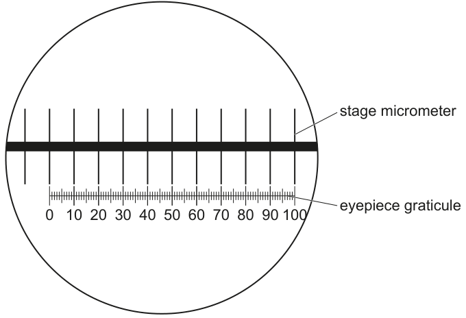
Use Fig. 2.3 to calculate the length of one eyepiece graticule unit.
Show your working.
Include the unit in your answer.
length of one eyepiece graticule unit = ______
Working
From Fig. 2.3, 10 eyepiece graticule units align with 1 division on the stage micrometer (the large tick marks on the upper scale).
One stage micrometer division = (given).
So:
Convert to micrometres:
Answer
Length of one eyepiece graticule unit = (= ).
(or )
Background Concept
An eyepiece graticule is a small glass disc with a scale etched onto it, sitting inside the eyepiece of a microscope. Because the eyepiece can be used with different objective lenses, the apparent size of one graticule division changes with magnification — the graticule itself does not have a fixed actual size. To use it for measurement, it must be calibrated against a stage micrometer, which is a slide with a scale of known actual length (each division is typically 0.1 mm or 0.2 mm, depending on the make).
Calibration procedure:
- Place the stage micrometer on the stage and focus on its scale.
- Rotate the eyepiece (without rotating the stage micrometer) until the two scales are parallel and overlap.
- Find two points where the two scales align exactly.
- Count how many eyepiece graticule units correspond to a known number of stage micrometer divisions.
- Divide the known stage micrometer length by the number of graticule units to get the actual length of one graticule unit at the current objective lens.
Understanding the Question
In Fig. 2.3 the two scales are aligned at the zero mark. The stage micrometer scale has large divisions; the eyepiece graticule has 100 small divisions numbered 0–100. One large division on the stage micrometer = (given).
The task is to find the actual length of one small division on the eyepiece graticule, showing the working and quoting the unit.
The mark scheme's first credited point is "10 eyepiece graticule units in " — i.e. one large tick on the stage micrometer aligns with 10 small ticks on the eyepiece graticule. This is the ratio needed.
Approach
Use the alignment ratio to convert a known length (one stage micrometer division) into the number of graticule units that span the same length, then take the length per graticule unit. The mark scheme rewards three points:
- State the alignment (10 graticule units in 0.2 mm).
- Divide 0.2 by 10.
- Quote the answer with the unit (mm or µm).
Step-by-Step Reasoning
-
Identify the alignment. In Fig. 2.3, the large tick marks on the stage micrometer are spaced apart such that one stage micrometer division covers 10 small divisions of the eyepiece graticule. This is the calibration ratio.
-
Substitute the known length. One stage micrometer division = . So 10 eyepiece graticule units = .
-
Divide to find the unit length.
-
Convert to a sensible unit (optional but conventional). Microscope measurements are usually quoted in micrometres:
The mark scheme accepts either or as the final answer. Both are correct and equivalent.
Key Takeaways
- The graticule has no fixed actual size; it must be calibrated at each magnification.
- The calibration procedure aligns the two scales and counts how many graticule units span a known stage micrometer length.
- — converting to µm is conventional for microscope measurements.
- Always show the working (the ratio you used and the division) — the mark scheme rewards the calculation, not just the final number.
Common Mistakes
- Reading the wrong number of aligned graticule units (e.g. using 5 or 20 instead of 10).
- Dividing the wrong way (e.g. dividing 10 by 0.2).
- Forgetting to include the unit in the final answer.
- Quoting the answer in the wrong unit (e.g. cm, nm) — both mm and µm are accepted; anything else is not.
- Omitting the working — the mark scheme explicitly rewards the substitution and the division, not just the final number.
Things to Be Careful About
- Read the alignment in Fig. 2.3 carefully: the stage micrometer has larger divisions than the graticule. Count the number of small graticule divisions that fit into one large stage micrometer division. In this calibration, that is 10.
- Show the working in the form the mark scheme rewards: the substitution (0.2 mm ÷ 10) and the result.
- The unit must accompany the numerical answer. mm and µm are the two accepted forms.
Fig. 2.4 shows the same eyepiece graticule and same lenses being used to measure the width of the section shown in Fig. 2.2.
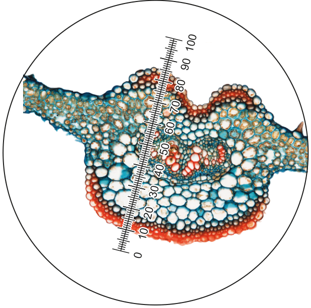
Use your answer in (b)(ii) to calculate the actual width of the section shown in Fig. 2.4.
Show your working.
actual width of the section = ______
Working
From Fig. 2.4, the width of the section spans 75 eyepiece graticule units (the graticule scale runs from 0 at one edge of the section to 75 at the other).
From (b)(ii), one eyepiece graticule unit = (or ).
Therefore:
Or, in micrometres:
Answer
Actual width of the section = (= ).
(or )
Background Concept
Once the eyepiece graticule has been calibrated at a given magnification, it can be used to measure any specimen viewed at the same objective lens on the same microscope. The procedure is:
- Replace the stage micrometer with the specimen slide (without changing the objective lens).
- Align the graticule scale across the feature to be measured.
- Read off the number of graticule units the feature spans.
- Multiply by the calibration factor (the actual length of one graticule unit, determined in the calibration step) to obtain the actual size.
This is exactly the relationship:
Understanding the Question
The graticule has already been calibrated in (b)(ii) at the magnification used in Fig. 2.4 (the same objective lens, since the same eyepiece graticule is being used). The question asks for the actual width of the section in Fig. 2.4, in mm or µm.
The mark scheme credits two points:
- State the correct number of eyepiece graticule units across the width of the section.
- Multiply that number by the answer to (b)(ii).
In Fig. 2.4 the graticule is positioned diagonally across the leaf section, with one end of the leaf at the 0 mark and the other end at the 75 mark, so the section spans 75 graticule units across its width.
Approach
Use the calibration factor from (b)(ii) ( per graticule unit, or per graticule unit) and the reading from Fig. 2.4 (75 units). Substitute into the relationship above and convert units as required.
Step-by-Step Reasoning
-
Read the graticule. In Fig. 2.4, the graticule is laid diagonally across the leaf section, going from 0 at the lower edge to 75 at the upper edge. The width of the section in graticule units is 75.
-
Apply the calibration. From (b)(ii), one eyepiece graticule unit = (= ) at this magnification. So:
Equivalently, in micrometres:
-
Check the unit consistency. The calibration was in mm (or µm), and the answer is in mm (or µm). No further conversion is needed. Both forms are accepted by the mark scheme.
Key Takeaways
- Once the graticule is calibrated, any specimen at the same magnification can be measured by reading the graticule and multiplying by the calibration factor.
- The unit of the calibration factor determines the unit of the answer. There is no need to convert again.
- The magnification must not change between calibration and measurement, or the calibration becomes invalid.
- Show the substitution — the mark scheme explicitly rewards seeing the multiplication, not just the final number.
Common Mistakes
- Reading the wrong number of graticule units (e.g. 70 or 80 instead of 75).
- Forgetting to multiply by the calibration factor and just quoting the graticule reading as the answer.
- Converting units incorrectly (e.g. quoting the answer in cm).
- Changing the magnification between calibration and measurement, then using the calibration factor anyway.
Things to Be Careful About
- The graticule is positioned diagonally across the section in Fig. 2.4 — read the value at the edge of the section (where the graticule line meets the leaf tissue), not at the centre.
- The answer must include a unit (mm or µm).
- Show the working as: number of units × calibration factor = actual size. The mark scheme requires seeing the multiplication.