Biology 9700/32 — May/June 2023
Cambridge AS Level · Advanced Practical Skills · worked solutions for every part, with the mark scheme
Topics Analysis, Conclusions and Evaluation · Manipulation, Measurement and Observation · Presentation of Data and Observations · Use of the Light Microscope
Grapes are fruit that contain high concentrations of soluble sugars such as sucrose, fructose and glucose.
The proportions of these sugars change as the grapes mature.
You will determine the concentration of reducing sugars in a sample of grape extract by using known concentrations of reducing sugar.
You are provided with the materials shown in Table 1.1.
Table 1.1
| labelled | contents | hazard | volume / |
|---|---|---|---|
| G | grape extract | none | 20 |
| W | distilled water | none | 100 |
| B | Benedict's solution | harmful irritant | 40 |
| R | 8.0% reducing sugar solution | none | 40 |
If any solution comes into contact with your skin, wash off immediately under cold water.
It is recommended that you wear suitable eye protection.
You will need to carry out a serial dilution of the 8.0% reducing sugar solution, R, to reduce the concentration by half between each successive dilution.
You will need to prepare four concentrations of reducing sugar in addition to 8.0% reducing sugar solution, R.
After the serial dilution is completed, you will need to have of each concentration available to use.
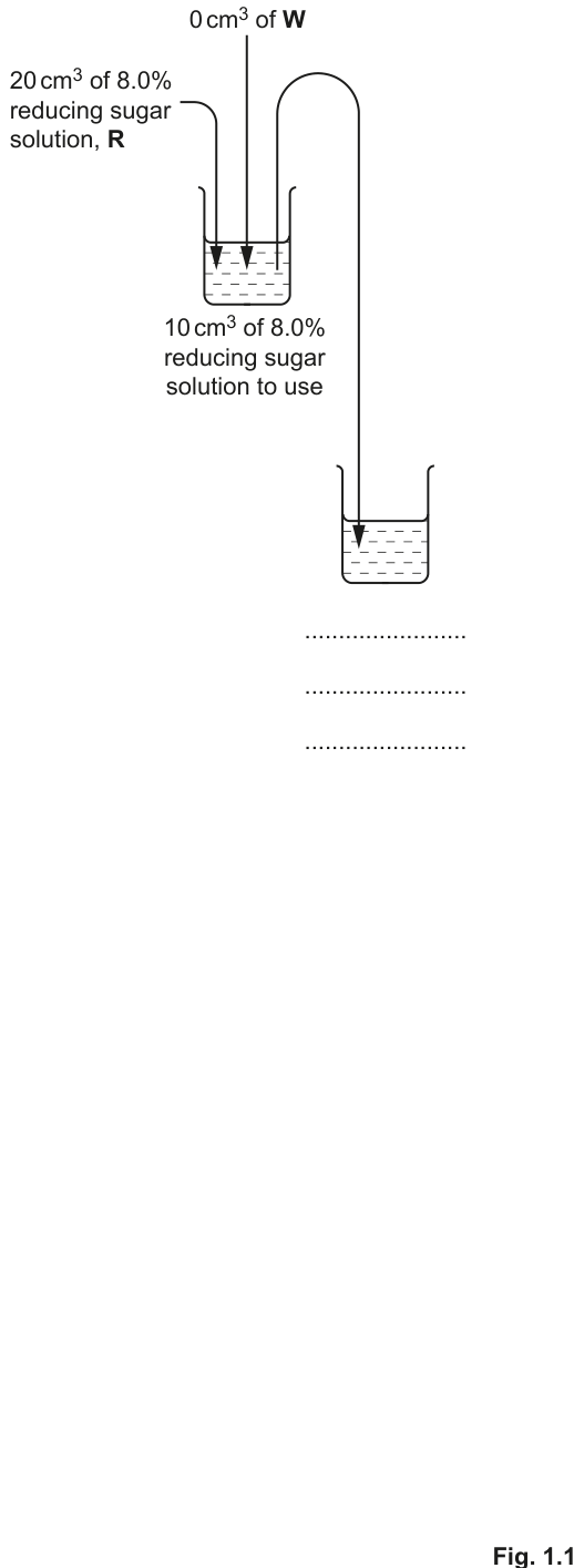
Complete Fig. 1.1 to show how you will prepare your serial dilution.
Fig. 1.1 shows the first two beakers you will use to make your serial dilution. You will need to draw three additional beakers.
For each beaker, add labelled arrows to show:
- the volume of reducing sugar solution transferred
- the volume of distilled water, W, added.
Under each beaker, state the concentration of reducing sugar solution.
Answer
Add three more beakers (beakers 3, 4 and 5) below beaker 2 in Fig. 1.1, each joined to the previous beaker by a curved transfer arrow. On each beaker draw two labelled arrows:
- the volume of reducing sugar solution transferred from the previous beaker (10 cm³ at every step)
- the volume of distilled water, W, added (10 cm³ added to each of beakers 2, 3, 4 and 5)
The first beaker already shows '0 cm³ of W' and contains the 20 cm³ of 8.0% solution, R.
Underneath the five beakers, the concentrations are:
| Beaker | Concentration of reducing sugar solution |
|---|---|
| 1 | 8.0% |
| 2 | 4.0% |
| 3 | 2.0% |
| 4 | 1.0% |
| 5 | 0.5% |
Each beaker contains 20 cm³ of solution; 10 cm³ is kept for use and 10 cm³ is transferred to the next beaker, where 10 cm³ of W is then added.
Five beakers: 8.0%, 4.0%, 2.0%, 1.0%, 0.5%, with 10 cm³ transferred from each beaker to the next and 10 cm³ of W added to each of beakers 2–5.
Background Concept
A serial dilution is a stepwise dilution in which the same dilution factor is applied at every step. Here the concentration is halved at each step (a 1-in-2 dilution), so starting from 8.0% the successive concentrations are 4.0%, 2.0%, 1.0% and 0.5%. To halve the concentration, equal volumes of stock solution and diluent (distilled water) are mixed.
Understanding the Question
The question stem already shows the first beaker, which contains 20 cm³ of the 8.0% stock solution R, and the second beaker, which is empty and ready to receive the first transfer. The student must add three more beakers, label the volumes transferred and added, and write the resulting concentration below each beaker. 10 cm³ of each concentration must be available for the Benedict's test in step 4, which is why each beaker contains 20 cm³ in total (10 cm³ kept for the test + 10 cm³ transferred to make the next dilution).
Approach
Work out the concentration at each step first, then annotate the diagram with the transfer volume (10 cm³) and the water volume (10 cm³) at every stage, and the percentage under each beaker.
Step-by-Step Reasoning
- Beaker 1: 20 cm³ of 8.0% R. 0 cm³ of W is added (already shown on the figure). Keep 10 cm³ for use; transfer 10 cm³ to beaker 2. Concentration under beaker 1: 8.0%.
- Beaker 2: receive 10 cm³ of 8.0% from beaker 1, add 10 cm³ of W. Total volume = 20 cm³. Concentration = (10/20) × 8.0% = 4.0%. Keep 10 cm³; transfer 10 cm³ to beaker 3. Under beaker 2: 4.0%.
- Beaker 3: receive 10 cm³ of 4.0%, add 10 cm³ of W. Total = 20 cm³. Concentration = 2.0%. Keep 10 cm³; transfer 10 cm³ to beaker 4. Under beaker 3: 2.0%.
- Beaker 4: receive 10 cm³ of 2.0%, add 10 cm³ of W. Total = 20 cm³. Concentration = 1.0%. Keep 10 cm³; transfer 10 cm³ to beaker 5. Under beaker 4: 1.0%.
- Beaker 5: receive 10 cm³ of 1.0%, add 10 cm³ of W. Total = 20 cm³. Concentration = 0.5%. Keep 10 cm³. Under beaker 5: 0.5%.
The arrows on the diagram should show 10 cm³ transferred at each step and 10 cm³ of W added to beakers 2–5. The % symbol must appear at least once.
Key Takeaways
- A halving serial dilution needs equal volumes of stock and water at each step.
- The total volume in each beaker must equal twice the volume kept, so that enough remains both for the test and for the next dilution.
- Always show the volumes transferred and added on the diagram, not just the final concentration.
Common Mistakes
- Halving the volume transferred instead of halving the concentration (e.g. transferring 5 cm³ instead of 10 cm³).
- Forgetting to add 10 cm³ of water to the new beaker before transferring the next aliquot.
- Writing the concentrations without the % symbol.
- Drawing the arrows in the wrong direction (e.g. showing water being removed instead of added).
Things to Be Careful About
- The first beaker already shows '0 cm³ of W' — do not add a water arrow to beaker 1.
- Each curved transfer arrow goes from the previous beaker to the next; the straight downward arrow with a label is the water addition.
- Make sure each of beakers 2, 3, 4 and 5 has BOTH a transfer arrow (10 cm³) and a water arrow (10 cm³).
Carry out step 1 to step 16.
step 1 Set up a water-bath and heat to boiling ready for step 6 and step 14.
step 2 Prepare the concentrations of reducing sugar solution as shown in Fig 1.1.
step 3 Label test-tubes with the concentrations shown in Fig. 1.1.
step 4 Put of the 8.0% reducing sugar solution into the appropriately labelled test-tube.
step 5 Put of Benedict's solution, B, into the same test-tube. Shake gently to mix.
step 6 Put this test-tube in the boiling water-bath. Start timing.
step 7 Measure the time taken to the first appearance of a colour change in the test-tube.
If there is no colour change after 120 seconds, stop timing and record as 'more than 120'.
step 8 Record the result from step 7 in 1(a)(ii).
step 9 Remove the test-tube from the water-bath. Put the test-tube in the test-tube rack.
step 10 Repeat step 4 to step 9 with the remaining concentrations of reducing sugar solution.
Record your results in an appropriate table for the known concentrations of reducing sugar.
Answer
Record the results in a table such as the one below (the actual times are the candidate's own observations; the values shown are representative examples only):
| Percentage concentration of reducing sugar | Time to first colour change / s |
|---|---|
| 8.0 | 22 |
| 4.0 | 38 |
| 2.0 | 60 |
| 1.0 | 85 |
| 0.5 | 110 |
Rules that must be followed to score the marks:
- The independent variable (percentage concentration of reducing sugar) heading comes first and carries no unit in the body of the table (the % is in the heading).
- The dependent variable (time to first colour change) heading includes both the quantity (time) and the unit (seconds or /s); the unit must NOT be repeated in the body of the table.
- All five concentrations are present.
- The time recorded for 8.0% is less than the time for 0.5% (the higher the sugar concentration, the faster the colour appears).
- Every time is a whole number of seconds (no decimals). If no colour has appeared by 120 s, record 'more than 120'.
Representative times such as 8.0% → 22 s, 4.0% → 38 s, 2.0% → 60 s, 1.0% → 85 s, 0.5% → 110 s (candidate's own values).
Background Concept
Benedict's reagent contains copper(II) sulfate in an alkaline solution. When heated with a reducing sugar, Cu²⁺ is reduced to Cu⁺, which precipitates as red copper(I) oxide. The higher the concentration of reducing sugar, the more Cu²⁺ is reduced and the faster the colour change (blue → green → yellow → orange → brick-red) becomes visible.
Understanding the Question
The candidate has prepared five concentrations of reducing sugar (8.0%, 4.0%, 2.0%, 1.0% and 0.5%) by serial dilution and is now performing the Benedict's test on each. Step 7 asks for the time to the first appearance of a colour change — the earliest visible sign that Cu²⁺ is being reduced, not the final brick-red colour. Step 8 asks the candidate to record that time in a results table.
Approach
Draw a two-column table. Put the independent variable (the concentration) in the left-hand column and the dependent variable (the time) in the right-hand column. Put units in the heading only, not in the body. Read each timing to the nearest whole second; if no colour has appeared by 120 s, write 'more than 120'.
Step-by-Step Reasoning
- Heading for the independent variable: 'Percentage concentration of reducing sugar' with the % symbol in the heading. Body cells contain numbers only (e.g. 8.0, 4.0, 2.0, 1.0, 0.5).
- Heading for the dependent variable: 'Time to first colour change' with the unit '/s' (or 'seconds') in the heading. Body cells contain whole numbers only.
- Trend: at 8.0% the colour change is fastest; at 0.5% it is slowest. The highest concentration must have a smaller time than the lowest concentration.
- Order: list the concentrations in descending order so the trend (decreasing time with increasing concentration) is visually obvious.
- Precision: record to the nearest whole second; the Benedict's colour change is judged by eye and sub-second precision is not meaningful.
Key Takeaways
- A results table must have a clear, descriptive heading for every column, with units in the heading and not in the body.
- The independent variable is listed first; the dependent variable follows.
- A simple monotonic trend (here, time decreases as concentration increases) should be visible from the table at a glance.
Common Mistakes
- Putting the unit (s, seconds, %) in the body of the table — the mark scheme rejects this.
- Reversing the order of the columns (time first, concentration second).
- Recording the time to the final brick-red colour rather than the first appearance of any change.
- Recording decimal times (e.g. 22.5 s) when the mark scheme requires whole seconds.
- Missing out one of the five concentrations.
Things to Be Careful About
- 'No colour change after 120 s' must be recorded as 'more than 120', not as a dash or as 120.
- Shake the tube gently after adding Benedict's to mix before heating; an unevenly mixed sample gives a misleadingly slow or patchy colour change.
- The water-bath must be at a rolling boil; if it is only just simmering, all the times are lengthened and the trend is preserved but the absolute values are not directly comparable with another group's data.
Identify one source of error in step 7.
Answer
The first appearance of a colour change is difficult to judge by eye — different observers (or the same observer on different occasions) will disagree on exactly when the first trace of green/yellow/orange appears.
Difficult to judge the first colour change.
Background Concept
Benedict's test does not switch sharply from blue to red; the colour passes through a continuous gradient of blue → green → yellow → orange → brick-red as more Cu²⁺ is reduced. The 'first appearance' of a change is therefore subjective and depends on the observer, the lighting, and the background against which the tube is viewed.
Understanding the Question
The question targets step 7 specifically, where the candidate has to start a stop clock when the test-tube goes into the bath and stop it at the first sign of a colour change. This is the most error-prone step in the whole procedure.
Approach
Identify ONE limitation that is intrinsic to the step itself, not a general lab error. The most direct answer is the subjectivity of judging the colour change.
Step-by-Step Reasoning
- The colour change is gradual, not instantaneous; there is no sharp endpoint.
- Lighting in the lab varies (overhead fluorescent vs. natural light from a window).
- The transition through green can be hard to distinguish from the original blue.
- Different people watching the same tube will stop the clock at different moments.
Any one of these captures the mark. The mark scheme accepts 'difficult to judge the first colour change'.
Key Takeaways
- A timing-based colour test always has subjectivity in the endpoint.
- Improvements that address this include: viewing the tube against a uniform white background, having the same person make all the readings, or replacing the eye judgement with a colorimeter that records absorbance at a fixed wavelength.
Common Mistakes
- Giving a general answer such as 'human error' or 'not accurate' — too vague to score.
- Naming a limitation that is not actually a fault of step 7 (e.g. 'the thermometer was unreliable' when no thermometer is used).
- Naming an improvement instead of an error.
Things to Be Careful About
- The question asks for ONE source of error. A second point, however correct, does not earn an extra mark here and can actually dilute the answer.
To determine the concentration of reducing sugar in grape extract G, you will need to test a sample of the extract.
State the volume of grape extract G that you will use to test for reducing sugars.
volume = ______
Answer
volume = 2 cm³
This matches the volume of reducing sugar solution used in step 4, so that the Benedict's-to-sample ratio is identical for G and the standards.
2 cm³
Background Concept
For the Benedict's test result to be comparable between the standards and the unknown, every variable other than the one being tested (the concentration of reducing sugar) must be kept the same. The volume of solution tested is one such variable.
Understanding the Question
Step 4 fixes the volume of standard reducing sugar solution at 2 cm³, and step 5 adds 2 cm³ of Benedict's reagent. To make the test on G directly comparable, the same 2 cm³ of grape extract must be used, with the same 2 cm³ of Benedict's reagent.
Approach
Read the controlled variable from the standard protocol: 2 cm³ of sample, 2 cm³ of Benedict's reagent. The same volume of grape extract is required.
Step-by-Step Reasoning
- The standards are tested with 2 cm³ of solution + 2 cm³ of Benedict's.
- G must be tested with the same volumes to give a comparable result.
- The volume to record is therefore 2 cm³.
Key Takeaways
- Controlled variables are the volumes of sample and reagent, the temperature of the water-bath, the timing method, and the same observer making the judgement.
- Any change in the volume tested would alter the ratio of Cu²⁺ to reducing sugar and invalidate the comparison with the calibration curve.
Common Mistakes
- Recording a different volume (e.g. 1 cm³ or 5 cm³) so that the G test is not directly comparable with the standards.
- Recording the volume with the wrong unit (e.g. ml instead of cm³).
Things to Be Careful About
- The mark scheme requires just the value, not a justification. A one-line answer of '2 cm³' is sufficient.
step 11 Label a test-tube G.
step 12 Transfer the volume of grape extract G that you stated in (a)(iv) into test-tube G.
step 13 Put of Benedict's solution, B, into the same test-tube. Shake gently to mix.
step 14 Put this test-tube in the boiling water-bath. Start timing.
step 15 Measure the time taken to the first appearance of a colour change in the test-tube.
If there is no colour change after 120 seconds, stop timing and record as 'more than 120'.
step 16 Record the result from step 15 in (a)(v).
Record the time taken for the first colour change in test-tube G.
time taken = ______
Answer
Record a time in whole seconds that lies between the times already obtained for 4.0% and 1.0% in the results table, e.g. (representative):
time taken = 52 s
(The actual value depends on the candidate's own timings. The mark requires the value to be in seconds and to be bracketed by the 4.0% and 1.0% times.)
e.g. 52 s (any whole-second value between the 4.0% and 1.0% times the candidate recorded)
Background Concept
The Benedict's test on G is the 'unknown' whose concentration we want to determine. Once the time has been recorded, the candidate will read the corresponding concentration off the calibration graph in (a)(vi)–(vii). For the read-off to fall inside the range of the standards, the time for G must lie between the times for the 4.0% and 1.0% standards — this is why the question has been designed with those two particular values in the dilution series.
Understanding the Question
Step 15 has been carried out and the candidate must now write the time on the answer line in (a)(v). The mark scheme requires a value in seconds that lies between the 4.0% and 1.0% results already in the table.
Approach
Look at the two bracketing times in the results table and pick a whole-second value between them. Record it with the unit s.
Step-by-Step Reasoning
- Find the 4.0% time in the table (e.g. 38 s) and the 1.0% time (e.g. 85 s).
- The G time must be a whole number of seconds in the open interval (38, 85) — for example 52 s, 60 s, 70 s, depending on the actual G extract.
- The unit is seconds (s). Do not write 'sec' or omit the unit.
Key Takeaways
- An unknown's value must fall inside the calibrated range; otherwise the calibration graph cannot be interpolated (or would require extrapolation, which is unreliable).
- The unit (s) is part of the answer.
Common Mistakes
- Writing a time outside the 4.0–1.0% bracket (e.g. faster than 4.0% or slower than 1.0%).
- Omitting the unit.
- Writing a decimal time when the protocol is timed in whole seconds.
- Writing 'more than 120' — that would mean G has less than 0.5% reducing sugar, which is implausible for a grape extract and would not allow the graph read-off to lie in the calibrated range.
Things to Be Careful About
- The candidate's own times for 4.0% and 1.0% are the bracketing values, not arbitrary numbers from this mark scheme.
The concentration of reducing sugars in G can be estimated from a graph of your results.
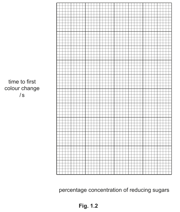
Draw a graph of the results you recorded in (a)(ii) on the grid in Fig. 1.2, using a line of best fit.
The axes have been labelled for you.
Use a sharp pencil.
Answer
On the grid in Fig. 1.2 (y-axis already labelled 'time to first colour change / s', x-axis already labelled 'percentage concentration of reducing sugars'):
- Choose a scale on the x-axis so that 2% occupies 2 cm; label every 2 cm (e.g. 0, 2, 4, 6, 8).
- Choose a scale on the y-axis that fits the candidate's own times (e.g. 0 to 120 s in 20 s intervals).
- Plot each of the five (concentration, time) points from the table using a small cross or a dot in a circle.
- Join the points with a thin, ruled line of best fit. The expected curve descends from upper-left to lower-right: as concentration increases, the time to first colour change decreases.
Descending curve from upper-left (low concentration, long time) to lower-right (high concentration, short time).
Background Concept
A calibration curve plots a known quantity (here, concentration of reducing sugar) on the x-axis against a measured response (here, time to first colour change) on the y-axis. The line of best fit summarises the relationship; once drawn, an unknown sample's response (the time recorded for G) can be read off horizontally to the line and then vertically down to the x-axis to obtain the concentration.
Understanding the Question
The y-axis label 'time to first colour change / s' and the x-axis label 'percentage concentration of reducing sugars' are already printed on Fig. 1.2. The candidate's task is to add the scales, the five plotted points, and the line of best fit.
Approach
Read the mark scheme requirements: x-axis scale of 2% per 2 cm labelled at least every 2 cm; y-axis scaled to suit the candidate's own times; thin ruled line of best fit. Then choose scales that use at least half the grid in both directions and are not awkward (no multiples of 3 or 7).
Step-by-Step Reasoning
- x-axis scale: 0, 2, 4, 6, 8 % (2% to 2 cm, labelled at every major line). 8% fits within ~8 cm of grid; 5 points span this range evenly.
- y-axis scale: pick the largest time from the table (e.g. 110 s or 120 s) and choose an interval that gives at least half the grid. 20 s intervals from 0 to 120 s works well; 10 s intervals from 0 to 60 s also work if the times are smaller.
- Plotting: each (concentration, time) pair becomes a small cross (×) or a circled dot (⊙) directly above the concentration and across from the time.
- Line of best fit: a single thin ruled line that passes through (or close to) all five points, with roughly equal numbers of points on each side. It is a smooth curve, not a series of straight segments. The curve descends — high concentration gives a fast colour change, so the line falls as we move right.
Key Takeaways
- A calibration curve must use scales that are easy to read and that use most of the grid.
- The line of best fit is a single smooth curve (or straight line) judged by eye; it should not be forced through every point or drawn as a series of connect-the-dots segments.
- Use a sharp pencil and a thin line so the marks can be awarded.
Common Mistakes
- Using awkward scales (e.g. 0, 3, 6, 9 on the x-axis) that make plotting difficult.
- Not using at least half the grid in one or both directions.
- Drawing the line as connect-the-dots (point-to-point) instead of a single best-fit line.
- Using a thick line or a felt-tip pen, which the mark scheme rejects.
- Forgetting to plot one of the five points.
Things to Be Careful About
- The y-axis interval must be chosen to suit the candidate's actual times, not a generic range. If all times are below 60 s, scale 0–60 in 10 s steps; if they reach 120 s, scale 0–120 in 20 s steps.
- The line of best fit is a curve here (Benedict's kinetics are non-linear) but a straight line is also acceptable if the data are nearly linear.
Use your graph to estimate the percentage concentration of reducing sugars in G.
Show on your graph how you determined your answer.
percentage concentration of reducing sugars in G = ______
Answer
On the graph in Fig. 1.2:
- Mark the time recorded for G (e.g. 52 s) on the y-axis.
- Draw a horizontal line from this point across to the line of best fit.
- From the intersection, draw a vertical line down to the x-axis.
- Read the concentration on the x-axis where the vertical line meets the axis.
Show all of these construction lines clearly on the graph (do not erase them). Then read off the value, e.g.:
percentage concentration of reducing sugars in G = 3.0% (representative)
e.g. 3.0% (the value read off the candidate's own graph; it depends on the G time recorded in (a)(v)).
Background Concept
Once a calibration curve is drawn, any unknown's response can be converted into a concentration by 'reading off' the graph: horizontal line from the response to the curve, then vertical line down to the concentration axis. This is called interpolation when the read-off lies inside the calibrated range, and extrapolation when it lies outside. Interpolation is reliable; extrapolation is unreliable because the curve may continue in a different manner outside the measured range.
Understanding the Question
The G time recorded in (a)(v) must be converted into a percentage concentration of reducing sugars. The candidate must show on the graph exactly how the value was obtained — the mark scheme awards one mark for the construction lines and one for the read-off value.
Approach
Use the standard 'L-shaped' construction: horizontal then vertical, with both lines drawn in pencil so the examiner can see the working.
Step-by-Step Reasoning
- Locate the G time on the y-axis (e.g. 52 s).
- Draw a horizontal pencil line rightwards until it meets the line of best fit.
- From that intersection, draw a vertical pencil line downwards until it meets the x-axis.
- Read the x-axis value at the foot of the vertical line. With representative data (8.0% → 22 s, 4.0% → 38 s, 2.0% → 60 s, 1.0% → 85 s, 0.5% → 110 s, G at 52 s) the read-off comes out around 3.0%.
- The G concentration should lie between 1.0% and 4.0% (because the G time was chosen to lie between the 1.0% and 4.0% times). If it falls outside, an arithmetic error has been made.
Key Takeaways
- Always show the construction lines on the graph; they are the evidence that the read-off is genuine.
- Interpolation between standards is reliable; extrapolation beyond the highest or lowest standard is not.
- The result should be quoted to a sensible number of significant figures — here one or two significant figures is appropriate.
Common Mistakes
- Erasing the construction lines after reading the value, leaving the examiner unable to verify the method.
- Reading off a value that is clearly outside the calibrated range (e.g. >8.0% or <0.5%) — a sign that the wrong axis has been used or the line has been extended by eye incorrectly.
- Quoting too many significant figures (e.g. 3.073%), implying a precision the method does not support.
- Forgetting the % symbol.
Things to Be Careful About
- The G concentration must be in the same units as the standards (percentage, %). Do not write 'g' or 'mol'.
- If the construction line falls between two minor gridlines, read to the nearest minor division and round sensibly.
Suggest how you would modify this investigation to obtain a more accurate estimate for the concentration of reducing sugars in sample G.
Answer
Any two of the following (or other creditworthy suggestions):
- Prepare more concentrations of reducing sugar close to the estimated value for G (e.g. 2.5%, 3.0%, 3.5%) so that the calibration curve has finer resolution in the critical region — the read-off becomes more accurate.
- Repeat each concentration (and the G test) several times and calculate a mean time, reducing the effect of random error in judging the first colour change.
- Hold a white card behind the test-tube when judging the first colour change, so that the background is uniform and the first appearance of green/yellow is easier to see.
Other creditworthy suggestions include: having the same observer make every reading to remove inter-observer variation, using a colorimeter to measure absorbance at a fixed wavelength instead of relying on eye judgement, and ensuring the water-bath is at a true rolling boil (control the temperature).
Any two of: more concentrations near the estimate; repeat and take a mean; use a white card behind the tube.
Background Concept
A 'more accurate' estimate can be achieved in two complementary ways: by reducing random error (variation between repeated readings) and by reducing systematic error (a bias in the method itself). Improvements to a method usually target one of these.
Understanding the Question
The candidate's estimate in (a)(vii) is based on a single timing for each standard and a single timing for G, with concentrations spaced at 1% intervals. The method therefore has two main weaknesses: the read-off is interpolated between widely spaced points, and the endpoint judgement is subjective.
Approach
List practical refinements that would tighten the calibration around the G value and tighten the endpoint judgement. Any two reasonable suggestions score the marks.
Step-by-Step Reasoning
- Finer calibration around the estimate: prepare extra standards at, say, 2.0%, 2.5%, 3.0%, 3.5%, 4.0% if the G estimate is around 3%. The line of best fit is then defined by more points in the critical region, so the read-off is more accurate.
- Replication and mean: time each standard (and G) three or more times and use the mean. Random variation in judging the colour change is averaged out, giving a more reproducible calibration curve.
- White card behind the tube: a uniform white background makes the first appearance of green or yellow against the original blue much easier to see, reducing subjectivity.
- Same observer for all readings: removes inter-observer bias.
- Colorimeter: measures absorbance at, say, 540 nm quantitatively; the time to reach a fixed absorbance can be measured objectively, removing all subjectivity.
- Standardised water-bath temperature: a thermostatically controlled bath at 100 °C rather than a variable-temperature beaker on a tripod makes the kinetics directly comparable between tubes.
Key Takeaways
- Improvements must be practical and specific. 'Be more careful' does not score; 'use a white card behind the tube' does.
- Each improvement should target a named limitation (random error, subjective endpoint, coarse calibration).
- Improvements that change the principle of the test (e.g. switching to a different reagent) are usually too large to score here.
Common Mistakes
- Vague answers: 'be more accurate', 'take more care', 'use better equipment' — the mark scheme rejects these.
- Suggesting an improvement that does not actually address a limitation of the method (e.g. 'use a different grape').
- Giving only one suggestion when the question is worth two marks.
Things to Be Careful About
- 'Repeat and find the mean' is the most universally applicable improvement and almost always scores.
- 'Use a white card behind the test-tube' is a Paper 3 classic — it costs nothing and visibly improves the endpoint judgement.
The concentration of reducing sugars in grapes changes as the grapes age (get older).
Table 1.2 shows the concentration of reducing sugars for grapes of different ages.
Table 1.2
| age of grapes / days | percentage concentration of reducing sugars |
|---|---|
| 14 | 1.1 |
| 28 | 1.9 |
| 42 | 2.6 |
| 56 | 3.9 |
| 70 | 7.5 |
| 84 | 11.3 |
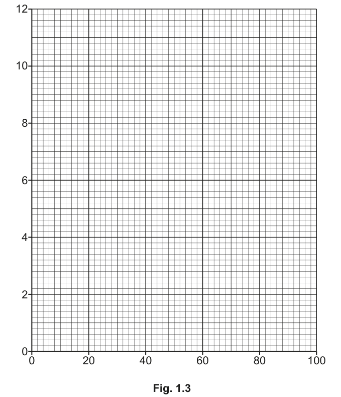
Plot a graph of the data shown in Table 1.2 on the grid in Fig. 1.3.
Answer
On the grid in Fig. 1.3:
- Label the x-axis: 'age of grapes / days' (or 'age of grapes' with 'days' in the heading).
- Label the y-axis: 'percentage concentration of reducing sugars'.
- The x-axis is pre-numbered 0 to 100 in steps of 20. The y-axis is pre-numbered 0 to 12 in steps of 2 — these scales are appropriate.
- Plot the six points from Table 1.2 using small crosses or dots in circles:
- (14, 1.1), (28, 1.9), (42, 2.6), (56, 3.9), (70, 7.5), (84, 11.3).
- (A line of best fit is not required by this part, but a smooth curve through the points is a sensible check on the data.)
Six plotted points: (14, 1.1), (28, 1.9), (42, 2.6), (56, 3.9), (70, 7.5), (84, 11.3).
Background Concept
A scatter graph is the standard way to display two continuous variables. Here the independent variable (age of grapes in days) goes on the x-axis and the dependent variable (percentage concentration of reducing sugars) on the y-axis. The y-axis is already pre-numbered 0 to 12 in steps of 2, and the x-axis 0 to 100 in steps of 20; these scales are appropriate for the data given.
Understanding the Question
The data are provided in Table 1.2. The candidate must add the two axis labels (with units in the heading, not in the body) and plot all six data points accurately.
Approach
Confirm the scales (already given), add the axis labels, and plot each (age, concentration) pair as a small cross or a circled dot, taking care to read each value to the nearest minor gridline.
Step-by-Step Reasoning
- x-axis label: 'age of grapes' with '/days' or 'days' in the heading. Each plotted point is centred on the appropriate age value.
- y-axis label: 'percentage concentration of reducing sugars' (no unit in the body; the % is in the heading).
- The y-axis is 0–12 in steps of 2, so values of 1.1, 1.9, 2.6, 3.9, 7.5 and 11.3 are all easily plotted.
- The points should be small (a cross of about 2 mm, or a dot of about 1 mm in a circle) so that the position is unambiguous.
- The points show a clear upward curve: reducing sugar concentration rises slowly at first and then more steeply between 56 and 84 days.
Key Takeaways
- Always put units in the axis label, not in the body of the graph.
- Use small, precise symbols (cross or circled dot); large blobs make the position ambiguous.
- Read each value to the nearest minor gridline; the y-axis here allows readings to the nearest 0.2 %.
Common Mistakes
- Putting the unit in the body of the graph (e.g. '14 days' on the x-axis) instead of in the heading.
- Plotting the points as large filled circles that obscure their true position.
- Missing one of the six points.
- Swapping the axes.
Things to Be Careful About
- The y-axis maximum is 12, so a value of 11.3 fits comfortably; if a candidate mistakenly extends the y-axis to 20, the curve becomes flat and the trend is hard to see.
Use your estimate from (a)(vii) and your graph in (b)(i) to estimate the age of the grapes that were used to make grape extract G.
age of grapes = ______
Answer
Using the concentration estimated in (a)(vii) (e.g. 3.0%):
- Mark this value on the y-axis of the graph in (b)(i).
- Draw a horizontal line from this point across to the curve.
- From the intersection, draw a vertical line down to the x-axis.
- Read the age in days where the vertical line meets the x-axis.
For a G concentration of 3.0%, the corresponding age is approximately:
age of grapes ≈ 50 days
(With the Table 1.2 data, 3.9% sits at 56 days and 2.6% sits at 42 days, so a concentration of 3.0% interpolates to roughly 50 days.)
e.g. 50 days (the value read off the candidate's own (b)(i) graph using their (a)(vii) estimate).
Background Concept
This part links the two graphs in the question. The (a)(vii) graph tells us the reducing-sugar concentration in G; the (b)(i) graph tells us how that concentration depends on the age of the grapes. Combining the two allows us to estimate the age of the grapes that produced G.
Understanding the Question
The candidate must take the concentration found in (a)(vii) and use it to read an age off the curve plotted in (b)(i). This is a second interpolation, this time of an age rather than a concentration.
Approach
Mark the concentration value on the y-axis of the (b)(i) graph, draw a horizontal line across to the curve, then a vertical line down to the x-axis, and read off the age. Show the construction lines on the graph.
Step-by-Step Reasoning
- The (a)(vii) estimate is, say, 3.0%.
- On the (b)(i) graph, the data show 2.6% at 42 days and 3.9% at 56 days. A concentration of 3.0% lies between these two points.
- Drawing horizontal and vertical construction lines, the vertical line meets the x-axis at roughly 50 days.
- The result is quoted to a sensible number of significant figures: 50 days, or about 7 weeks.
Key Takeaways
- The two graphs in the question are designed to be used together: the (a) calibration converts time → concentration; the (b) curve converts concentration → age.
- The age read-off should be inside the calibrated age range (14–84 days). If the (a)(vii) estimate is outside the range 1.1–11.3%, the read-off would require extrapolation and would be unreliable.
- Construction lines must be left on the graph so the examiner can see the working.
Common Mistakes
- Forgetting to use the candidate's own (a)(vii) estimate, and using someone else's value instead.
- Drawing the construction lines in the wrong order (vertical first, then horizontal).
- Quoting the age to unrealistic precision (e.g. 49.7 days).
- Forgetting the unit 'days'.
Things to Be Careful About
- The relationship between age and reducing-sugar concentration is non-linear (the curve steepens with age), so a simple linear interpolation between 42 and 56 days slightly underestimates the age at 3.0%. A construction line drawn on the actual curve gives a slightly different (and more correct) answer.
Grapes contain starch as well as reducing sugars. In a study, the concentration of amylase in grapes was measured as the grapes aged.
The results of the study are shown in Fig. 1.4.
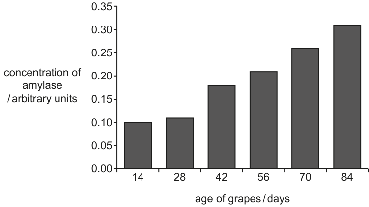
Use the data in Fig. 1.3 and Fig. 1.4 to suggest a possible explanation for the change in the concentration of reducing sugars in grapes as they age.
Answer
- The concentration of amylase in the grapes increases as the grapes age (Fig. 1.4).
- The concentration of reducing sugars in the grapes also increases as the grapes age (Fig. 1.3 / Table 1.2).
- Amylase hydrolyses starch (a storage polysaccharide in the grapes) into reducing sugars (maltose and glucose).
- Therefore, as the grapes age and produce more amylase, more starch is broken down into reducing sugars, leading to the observed rise in reducing-sugar concentration.
Both amylase and reducing-sugar concentration increase as grapes age; amylase hydrolyses starch to reducing sugars, so more amylase → more reducing sugars.
Background Concept
Starch is a storage polysaccharide made of α-glucose units joined by α-1,4 (and some α-1,6) glycosidic bonds. Amylase is a hydrolytic enzyme that breaks these bonds, releasing maltose (a disaccharide reducing sugar) and free glucose. In a ripening fruit, stored starch is progressively converted to soluble sugars; this is what makes ripe fruit sweet. The enzyme and the product therefore rise together.
Understanding the Question
The candidate is given two figures: Fig. 1.3 (or its data table) shows reducing-sugar concentration rising with grape age; Fig. 1.4 shows amylase concentration also rising with grape age. The question asks for a biological explanation that links the two trends.
Approach
State the trend in each figure, name the substrate and the product of amylase action, and then connect the rising amylase concentration to the rising reducing-sugar concentration.
Step-by-Step Reasoning
- Trend in Fig. 1.4: amylase concentration rises from ~0.10 arbitrary units at 14 days to ~0.31 arbitrary units at 84 days. More amylase is present in older grapes.
- Trend in Fig. 1.3 / Table 1.2: reducing-sugar concentration rises from 1.1% at 14 days to 11.3% at 84 days. Older grapes contain more reducing sugar.
- Enzyme action: amylase hydrolyses the α-1,4 glycosidic bonds of starch, producing maltose and glucose — both of which are reducing sugars.
- Link: the more amylase present, the more starch is hydrolysed per unit time, and so the more reducing sugar accumulates in the grape.
- Conclusion: the rise in reducing-sugar concentration as grapes age is explained, at least in part, by the parallel rise in amylase concentration, which converts stored starch into soluble reducing sugars.
Key Takeaways
- The two figures show a co-variation: both variables increase with age. Co-variation is consistent with a causal link, although it does not prove one — the explanation needs the biological mechanism (amylase hydrolysing starch) as well as the correlation.
- Amylase is a hydrolytic enzyme; the products of starch hydrolysis (maltose and glucose) are reducing sugars and so would give a positive Benedict's test.
- This is the same chemistry that underlies the ripening of bananas (starch → sugar), the malting of barley in brewing, and the digestion of starch in the human gut.
Common Mistakes
- Stating only the trends without giving the mechanism — the mark scheme requires the link 'amylase hydrolyses starch' to be made explicit.
- Stating the mechanism but not linking it to the change in reducing-sugar concentration.
- Confusing the substrate and product: 'amylase breaks down reducing sugars' (wrong direction) or 'amylase makes starch' (the opposite of its real action).
- Confusing amylase with a different enzyme (e.g. saying it hydrolyses sucrose) — the question specifically says grapes contain starch, so the substrate is starch.
Things to Be Careful About
- The mark scheme awards 3 marks: (1) both amylase and reducing sugar increase with age, (2) amylase hydrolyses starch to reducing sugars, (3) more amylase → more reducing sugar. All three must be present in the answer.
- Use the precise biological terms: 'hydrolyses' (or 'hydrolyses the glycosidic bonds of'), 'starch', 'reducing sugars' (maltose and glucose are both acceptable as named examples).
The rest of this paper
1 more questions- Q2Use of the Light Microscope · Analysis, Conclusions and Evaluation17M