Biology 9700/35 — October/November 2020
Cambridge AS Level · Advanced Practical Skills · worked solutions for every part, with the mark scheme
Topics Analysis, Conclusions and Evaluation · Manipulation, Measurement and Observation · Presentation of Data and Observations · Use of the Light Microscope
Sucrase is an enzyme which hydrolyses the disaccharide sucrose into reducing sugars, as shown in Fig. 1.1.
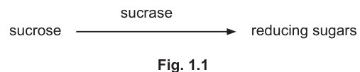
Fig. 1.1
The progress of this reaction can be followed by measuring the concentration of reducing sugar produced. To do this, samples can be taken at time intervals and the action of sucrase stopped in the sample.
The concentration of reducing sugar in the sample can then be tested using Benedict’s solution and compared to known concentrations of reducing sugar.
You are provided with the materials shown in Table 1.1.
Table 1.1
| labelled | contents | hazard | volume / |
|---|---|---|---|
| R | 2.0% reducing sugar solution | none | 50 |
| B | Benedict’s solution | harmful irritant | 25 |
| W | distilled water | none | 150 |
| U | unknown concentration of reducing sugar, sampled at 2 minutes | harmful irritant | 2 |
If any solution comes into contact with your skin, wash off immediately under cold water.
It is recommended that you wear suitable eye protection.
You need to carry out a serial dilution of the 2.0% reducing sugar solution, R, to reduce the concentration by half between each successive dilution.
Fig. 1.2 shows the first two beakers you will use to make your serial dilution.
Complete Fig. 1.2 by drawing as many extra beakers as you need for your serial dilution.
For each beaker:
- state, under the beaker, the volume and concentration of reducing sugar solution available for use in the investigation
- use one arrow with a label, above the beaker, to show the volume and concentration of reducing sugar solution added to prepare the concentration
- use another arrow with a label, above the beaker, to show the volume of W added to prepare the concentration.
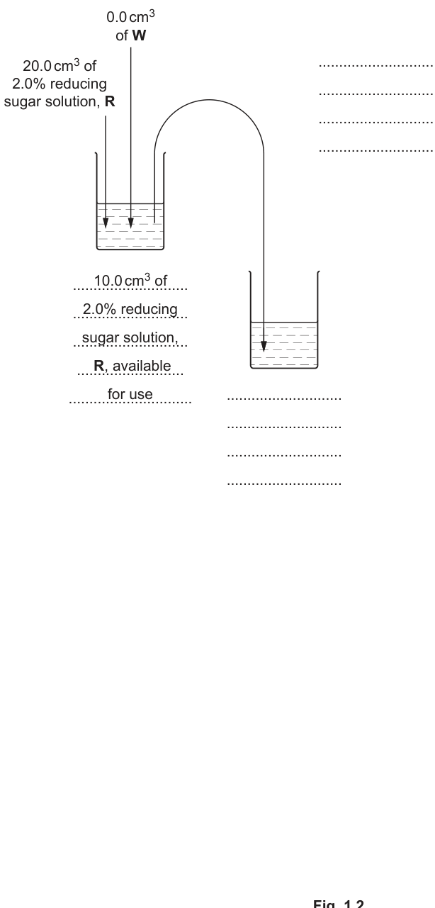
Fig. 1.2
Answer
Complete Fig. 1.2 by labelling the second beaker as 1.0% and adding three more beakers to the right. Each new beaker must show a curved transfer arrow of 10 cm³ from the previous beaker (labelled with the volume and concentration of reducing sugar solution added) and a vertical arrow of 10 cm³ of W added (labelled with the volume).
The concentration labelled under each beaker (left to right) is: 2.0% (already shown), 1.0%, 0.5%, 0.25%, 0.125%.
For each new beaker the volume of reducing-sugar solution transferred from the previous beaker is 10 cm³, and the volume of W added is 10 cm³. The label below each beaker states '10.0 cm³ of [X]% reducing sugar solution, available for use'.
Three further beakers at 0.5%, 0.25% and 0.125% (and the second beaker labelled 1.0%), each made by adding 10 cm³ of the previous concentration and 10 cm³ of W.
Background Concept
A serial dilution is a stepwise dilution in which each new concentration is prepared by transferring a fixed volume from the previous dilution and adding a fixed volume of diluent. When the volumes of solution and diluent are equal, the concentration is halved at each step. The same volume (here 10 cm³) is taken forward each time, so only the concentration changes.
Understanding the Question
Fig. 1.2 already shows the first beaker (20.0 cm³ of 2.0% reducing sugar solution R, 0.0 cm³ of W added, 10.0 cm³ of 2.0% 'available for use') and the start of the second beaker (a curved arrow showing 10.0 cm³ being transferred in). The candidate must complete the diagram by labelling the second beaker, showing 10 cm³ of W added to it, and drawing as many further beakers as needed for the Benedict's test calibration.
Approach
The halving sequence starting at 2.0% is 2.0% → 1.0% → 0.5% → 0.25% → 0.125%. Two beakers are already started (2.0% and 1.0%), so three more beakers are needed for 0.5%, 0.25% and 0.125%. At each step, transfer 10 cm³ of the previous concentration into the next beaker and add 10 cm³ of W; this doubles the volume (20 cm³ total) and halves the concentration.
Step-by-Step Reasoning
The mark scheme awards three points:
-
Concentration labels under the correct sequence of beakers — 1.0%, 0.5%, 0.25% and 0.125% must appear, with the % sign used at least once. The 1.0% label goes under the second beaker (which is drawn but unlabelled in the question). The 0.5%, 0.25% and 0.125% labels go under the three new beakers.
-
Transfer arrow — each new beaker must show 10 cm³ of the previous concentration being transferred in, with cm³ written at least once. The curved arrow from the previous beaker is the standard convention.
-
Water addition — each new beaker must show 10 cm³ of W being added, with cm³ written at least once. A vertical arrow into the beaker is the standard convention.
A typical completed diagram has five beakers in a row, with curved transfer arrows going from each beaker to the next, vertical arrows of 10 cm³ of W into each new beaker, and labels below each beaker such as '10.0 cm³ of 0.5% reducing sugar solution, available for use'.
Key Takeaways
- A halving serial dilution uses equal volumes of solution and diluent, so each step halves the concentration.
- Five beakers in total (2.0%, 1.0%, 0.5%, 0.25%, 0.125%) give a useful range for a Benedict's test calibration.
- Labelling must include units (cm³) and the percentage sign (%) at least once.
Common Mistakes
- Forgetting the % sign in the concentration labels.
- Drawing only two beakers (so the lowest concentration is 0.5%, which is too concentrated to give a useful range for the unknown).
- Showing the wrong volume of W (e.g. 5 cm³, which would not halve the concentration).
- Putting the wrong concentration under a beaker (e.g. labelling the third beaker 0.25% instead of 0.5%).
- Omitting the 'available for use' volume label below each beaker.
Things to Be Careful About
- The 1.0% label must be written under the second beaker (already drawn), not just under the new beakers.
- The unit 'cm³' must appear with both the transfer and the water-addition volumes.
- Only 10.0 cm³ is taken forward at each step; the other 10 cm³ remains in the beaker, which is why each beaker holds 20 cm³ in total.
Carry out step 1 to step 8.
- Set up a water-bath and heat to boiling ready for use in step 6.
- Prepare the concentrations of reducing sugar solution decided in (a)(i) and shown in Fig. 1.2. Use a glass rod to mix the reducing sugar solutions and water.
- Label test-tubes with the concentrations of reducing sugar solution prepared in step 2.
- Put of each concentration of reducing sugar solution into an appropriately labelled test-tube.
- Put of Benedict’s solution, B, into each of these test-tubes. Shake gently to mix.
- Put the test-tube labelled 2.0% into the boiling water-bath. Start timing.
- Measure the time taken to the first colour change. Record the result in (a)(ii). If there is no colour change after 90 seconds, record as ‘more than 90’.
- Repeat step 6 and step 7 using each of the concentrations of reducing sugar solution you prepared in step 2, instead of 2.0%. Record your results in (a)(ii).
Record your results in an appropriate table.
Answer
| percentage concentration of sugar | time / s |
|---|---|
| 2.0 | 25 |
| 1.0 | 35 |
| 0.5 | 50 |
| 0.25 | 70 |
| 0.125 | 85 |
(Representative values; the candidate's own times will depend on their bench. The trend must be that time decreases as concentration increases.)
Table with heading 'percentage concentration of sugar' (independent variable) and 'time / s' (dependent variable), no units in the body, times for all five concentrations showing a decrease in time as concentration increases, recorded to the nearest whole second.
Background Concept
The Benedict's test detects reducing sugars. When Benedict's solution is heated with a reducing sugar, the blue Cu(II) ions are reduced to red Cu(I) oxide. A higher concentration of reducing sugar produces a faster and more intense colour change. The time taken for the first appearance of the colour change is therefore inversely related to the concentration of reducing sugar in the sample.
Understanding the Question
The candidate has prepared the five concentrations of reducing sugar solution (2.0%, 1.0%, 0.5%, 0.25%, 0.125%) decided in (a)(i) and is performing the Benedict's test on each one (steps 1-8). They must record their results in a table that is laid out correctly and shows the expected trend.
Approach
Construct a two-column table with the independent variable (concentration of reducing sugar) on the left and the dependent variable (time to first colour change) on the right. Use a heading that includes the quantity and the unit for the dependent variable, and put the unit in the heading rather than repeating it in the body of the table. Record each time to the nearest whole second.
Step-by-Step Reasoning
The mark scheme awards five points:
-
Heading for the independent variable — 'percentage concentration of sugar' (or equivalent). This heading must come before the heading for the dependent variable. No units in the body of the table.
-
Heading for the dependent variable — 'time' with the unit 's' or 'seconds'. No units in the body of the table.
-
Times for all concentrations — every concentration (2.0%, 1.0%, 0.5%, 0.25%, 0.125%) must have a time recorded.
-
Correct trend — the time must decrease as the concentration increases (more reducing sugar → faster colour change).
-
Results to the nearest whole second — no decimals, no 'more than 90' if a real time was measured (the 'more than 90' option is only used when there really was no colour change within 90 s).
A representative set of results is shown above. The exact values are not the point; the format, the units, the trend and the precision are what earn the marks.
Key Takeaways
- The Benedict's test gives a faster colour change at higher reducing-sugar concentrations, so time is inversely related to concentration.
- CIE table conventions: the heading includes the quantity and the unit; the body contains only the numbers.
- The independent-variable heading comes before the dependent-variable heading in a CIE table.
Common Mistakes
- Repeating the unit (e.g. '%' or 's') in the body of the table.
- Recording the time in minutes instead of seconds.
- Recording the trend the wrong way round (time increasing with concentration).
- Recording a decimal time (e.g. 35.5 s) instead of a whole number.
- Using the 'more than 90' option for a concentration that did give a colour change.
Things to Be Careful About
- The candidate's times will not match the representative values above; the marks are for the conventions and the trend, not the specific numbers.
- The 'more than 90' option is only used when no colour change is observed within 90 s; for the concentrations used here, a colour change should occur within 90 s for all five.
- The table should be ruled neatly with clear column headings.
You are provided with an unknown concentration of reducing sugar solution in the test-tube labelled U.
- Put of B into the test-tube labelled U.
- Repeat step 6 to step 7, using the test-tube labelled U instead of 2.0%. Record your result for U in (a)(iii).
Record your result for U.
result for U = ______
Answer
result for U = 60 s (representative value)
(The candidate's own time will depend on their bench; the unit 's' or 'seconds' is required for the mark.)
60 s (representative)
Background Concept
The Benedict's test is performed on the unknown U in exactly the same way as on the standard concentrations in (a)(ii): 2 cm³ of B is added, the tube is heated in a boiling water bath, and the time to the first colour change is recorded.
Understanding the Question
After recording the calibration times in (a)(ii), the candidate performs the Benedict's test on the unknown U and records the time in the space provided.
Approach
Record the time to the nearest whole second, with the unit 's' (or 'seconds'). The candidate's actual time will depend on their bench and on the concentration of U; the mark is for the format, not the value.
Step-by-Step Reasoning
The mark scheme requires:
- The time recorded (a number).
- The unit 's' or 'seconds'.
A representative time of 60 s is used here for illustration; the candidate's value will be whatever they measure.
Key Takeaways
- The Benedict's test on U uses the same procedure as on the standards; the time is recorded to the nearest whole second.
- The unit 's' must be written, not just a bare number.
Common Mistakes
- Writing the time without the unit.
- Writing the time in minutes instead of seconds.
- Using 'more than 90' when a colour change was actually observed.
Things to Be Careful About
- The exact value of the time is not the point; the mark is for the recording conventions.
- The candidate should use the same stopwatch and judgement of 'first colour change' that they used for the standards in (a)(ii).
Using your results in (a)(ii) and (a)(iii), estimate the concentration of reducing sugars in U.
U = ______
Answer
U = 0.4 % (representative value)
(If U gave 60 s, this falls between the 0.5% standard (50 s) and the 0.25% standard (70 s), so by linear interpolation the concentration is approximately 0.4 %. The candidate's own value will depend on their results in (a)(ii) and (a)(iii).)
0.4 % (representative)
Background Concept
The results in (a)(ii) form a calibration table: each known concentration of reducing sugar has a measured time to the first colour change. The unknown U has a measured time, and its concentration can be estimated by finding the standard whose time is closest to (or by interpolating between the two standards on either side of) the time for U.
Understanding the Question
The candidate has a time for U from (a)(iii) and a calibration table from (a)(ii). They must use these to estimate the concentration of reducing sugars in U.
Approach
Find the two standards in the calibration table whose times bracket the time for U, then interpolate to estimate the concentration. If the time for U exactly matches a standard, use that concentration. If it falls between two standards, estimate the concentration as lying between the two.
Step-by-Step Reasoning
In the representative example, U gave 60 s. The calibration table is:
- 2.0 % → 25 s
- 1.0 % → 35 s
- 0.5 % → 50 s
- 0.25 % → 70 s
- 0.125 % → 85 s
60 s falls between 0.5 % (50 s) and 0.25 % (70 s). By linear interpolation, the concentration is approximately 0.5 % − (60 − 50)/(70 − 50) × (0.5 % − 0.25 %) = 0.5 % − 0.5 × 0.25 % = 0.5 % − 0.125 % = 0.375 % ≈ 0.4 %.
The mark is awarded for any reasonable estimate that is consistent with the candidate's own results. The candidate should not write a value that has no basis in their data.
Key Takeaways
- A calibration table allows an unknown concentration to be estimated by matching the measured time to the time of a standard.
- Interpolation between two bracketing standards gives a more precise estimate than just picking the nearest standard.
- The estimate must be consistent with the candidate's own measurements, not with the representative values used here.
Common Mistakes
- Quoting a value with no basis in the candidate's own data (e.g. giving 0.5 % when U clearly took a different time from the 0.5 % standard).
- Giving an estimate outside the range of the standards (e.g. > 2.0 % or < 0.125 %).
- Forgetting to include the % sign.
Things to Be Careful About
- The exact estimate is not the point; the mark is for using the calibration data to make a reasonable estimate.
- The candidate should write the value with the % sign, not as a bare number.
Suggest how you would make improvements to this investigation to obtain a more accurate estimate of the concentration of reducing sugars in U.
Answer
Any two from:
- Prepare additional reducing-sugar concentrations between the two standards that lie on either side of the estimated value of U (e.g. 0.3 % and 0.4 %), and repeat the Benedict's test on these, to obtain a more precise interpolation.
- Use a single-step (proportional) dilution from the 2.0 % stock for each standard, rather than a serial dilution, to avoid the accumulation of pipetting error across multiple steps.
- Plot a calibration graph of time against concentration for the known standards, then read off the concentration of U from its time on the graph.
Any two of: (1) more concentrations bracketing the estimate; (2) single-step proportional dilution; (3) plot a calibration graph and read off the value.
Background Concept
The accuracy of an estimate from a calibration table depends on:
- The number of standards in the region of the estimate (more standards → better interpolation).
- The accuracy of the standards themselves (cumulative pipetting error in a serial dilution makes the later standards less accurate).
- The method of reading the calibration (a graph allows more precise reading than a table).
Understanding the Question
The candidate has estimated the concentration of U from a five-standard serial dilution, but the estimate is only as good as the resolution of the calibration in the region of U. They are asked to suggest how the procedure could be improved to give a more accurate estimate.
Approach
Identify the main sources of error in the current procedure and suggest specific, practical improvements that address them.
Step-by-Step Reasoning
The mark scheme offers three creditworthy improvements; any two earn the marks:
-
More concentrations around the estimate — the current standards are 2.0 %, 1.0 %, 0.5 %, 0.25 % and 0.125 %. If U has a concentration of, say, 0.4 %, then the two bracketing standards are 0.5 % and 0.25 %, and the gap is 0.25 %. Adding standards at 0.3 % and 0.4 % (or 0.35 % and 0.45 %) would allow a much more precise interpolation.
-
Proportional (single-step) dilution — in a serial dilution, the error in each step accumulates. For example, if the 0.5 % standard is slightly off, then the 0.25 % and 0.125 % standards are also off. A single-step dilution from the 2.0 % stock for each standard avoids this accumulation.
-
Plot a calibration graph — reading a value from a continuous graph is more precise than matching a time to the nearest standard in a table. The graph of time against concentration can be used to read off the concentration of U.
Key Takeaways
- The accuracy of a calibration depends on the number and accuracy of the standards.
- Serial dilutions accumulate error; single-step dilutions do not.
- A calibration graph gives a more precise read-off than a table.
Common Mistakes
- Suggesting vague improvements that do not address a specific source of error (e.g. 'be more careful', 'repeat the experiment').
- Suggesting an improvement that is not practical for this procedure (e.g. 'use a colorimeter' — the method here is a visual judgement of first colour change, not a colorimeter reading).
- Repeating the same idea in two different forms and counting it as two improvements.
Things to Be Careful About
- Each improvement should be specific and address a particular limitation of the procedure.
- 'More repeats' or 'more concentrations' alone is not enough; the improvement must be tied to the calibration (e.g. 'more concentrations in the region of the estimate').
- The mark scheme says 'any two', so two specific improvements earn both marks.
A student wanted to determine the Michaelis-Menten constant () for sucrase during the hydrolysis of sucrose, as shown in Fig. 1.1.
The student measured the initial rate of reaction at different concentrations of sucrose.
The results are shown in Fig. 1.3.
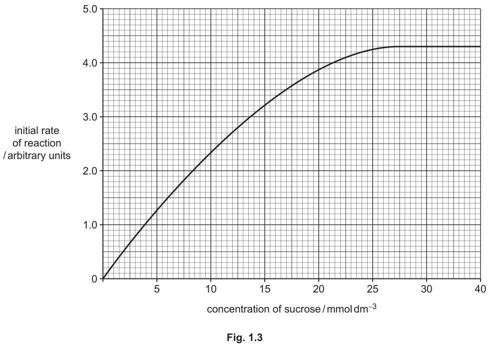
Fig. 1.3
Use the graph in Fig. 1.3 to estimate the Michaelis-Menten constant ().
Show your working on the graph and in the space below.
= ______
Working
- Read the maximum initial rate (Vmax) from the plateau of the curve in Fig. 1.3: Vmax ≈ 4.3 au.
- Calculate 1/2 Vmax: 1/2 × 4.3 = 2.15 au.
- Read the sucrose concentration on the x-axis that corresponds to an initial rate of 2.15 au on the curve: K_m ≈ 8 mmol dm⁻³.
Answer
K_m = 8 mmol dm⁻³
K_m ≈ 8 mmol dm⁻³
Background Concept
The Michaelis-Menten constant K_m is the substrate concentration at which the initial rate of an enzyme-catalysed reaction is half of the maximum rate (Vmax). It is a measure of the affinity of the enzyme for its substrate: a low K_m indicates high affinity (the enzyme reaches half Vmax at a low substrate concentration), and a high K_m indicates low affinity.
On a graph of initial rate against substrate concentration, the curve rises steeply at first and then levels off at Vmax. The K_m is read off the curve as the x-coordinate at which the y-coordinate is 1/2 Vmax.
Understanding the Question
Fig. 1.3 shows the initial rate of the sucrase reaction (in arbitrary units) plotted against the sucrose concentration (in mmol dm⁻³). The curve plateaus at a Vmax of about 4.3 au. The candidate must read Vmax, calculate 1/2 Vmax, and then read the corresponding x-value to find K_m.
Approach
Three steps on the graph:
- Mark the plateau and read Vmax on the y-axis.
- Halve this value to get 1/2 Vmax.
- Draw a horizontal line from 1/2 Vmax on the y-axis to the curve, then drop a vertical line from that point to the x-axis; the x-coordinate is K_m.
Step-by-Step Reasoning
The mark scheme awards three points:
-
Vmax read correctly from the graph at 4.3 au — the curve plateaus at 4.3 au, so Vmax = 4.3 au.
-
1/2 Vmax calculated correctly — 1/2 × 4.3 = 2.15 au.
-
K_m read off the graph — drawing a horizontal line from 2.15 au to the curve, then dropping to the x-axis, gives a value of approximately 8 mmol dm⁻³. (The exact value depends on how carefully the line is drawn, but 7-9 mmol dm⁻³ is the creditworthy range.)
The candidate should mark the Vmax plateau on the graph, draw a horizontal line at 1/2 Vmax, and then read the K_m from the x-axis. They should also show the working in writing below the graph.
Key Takeaways
- K_m is the substrate concentration at which the initial rate is half of Vmax.
- On a Michaelis-Menten curve, Vmax is the plateau value and K_m is the x-value at 1/2 Vmax.
- A larger K_m means lower enzyme-substrate affinity.
Common Mistakes
- Reading Vmax as the y-value at the highest x shown (40 mmol dm⁻³) rather than the plateau value.
- Confusing K_m with Vmax (writing the y-value instead of the x-value).
- Using 1/2 of the x-axis maximum instead of 1/2 Vmax (i.e. using 20 mmol dm⁻³ instead of finding where the rate is 2.15 au).
- Forgetting the unit (mmol dm⁻³).
Things to Be Careful About
- The candidate's value of K_m will depend on how carefully they draw the horizontal and vertical lines; a range of 7-9 mmol dm⁻³ is acceptable.
- The working must be shown on the graph as well as in writing; the mark scheme expects to see the construction lines.
- The unit (mmol dm⁻³) must accompany the numerical value.
The value for another enzyme, Z, is .
State which enzyme, Z or sucrase, has a lower affinity for its substrate.
Give a reason for your answer.
enzyme = ______
reason = ______
Answer
enzyme = sucrase
reason = K_m is higher for sucrase (≈ 8 mmol dm⁻³) than for enzyme Z (0.95 mmol dm⁻³), so sucrase has a lower affinity for its substrate.
sucrase; K_m is higher for sucrase than for enzyme Z, so sucrase has a lower affinity for its substrate.
Background Concept
K_m is inversely related to enzyme-substrate affinity:
- A low K_m means the enzyme reaches half Vmax at a low substrate concentration, indicating a high affinity (the enzyme binds substrate efficiently even when it is scarce).
- A high K_m means the enzyme needs a high substrate concentration to reach half Vmax, indicating a low affinity (the enzyme binds substrate less efficiently).
Understanding the Question
The K_m of sucrase has been estimated from Fig. 1.3 in (b)(i) (≈ 8 mmol dm⁻³), and the K_m of enzyme Z is given as 0.95 mmol dm⁻³. The candidate must state which enzyme has the lower affinity for its substrate and give a reason.
Approach
Compare the two K_m values: the enzyme with the higher K_m has the lower affinity.
Step-by-Step Reasoning
K_m(sucrase) ≈ 8 mmol dm⁻³ > K_m(Z) = 0.95 mmol dm⁻³.
So sucrase has the higher K_m, and therefore the lower affinity for its substrate.
The mark scheme requires:
- Identification of sucrase as the enzyme with the lower affinity.
- The reason: K_m is higher for sucrase (than for Z).
Both points are needed for the single mark.
Key Takeaways
- K_m is inversely related to enzyme-substrate affinity.
- The higher the K_m, the lower the affinity.
- To compare two enzymes, compare their K_m values: the larger K_m indicates the lower affinity.
Common Mistakes
- Identifying enzyme Z as having the lower affinity (this would be wrong; Z has the lower K_m, so it has the higher affinity).
- Stating the reason as 'sucrase is slower' or 'sucrase has a higher Vmax' (irrelevant to the K_m comparison).
- Stating only that sucrase has a lower affinity without giving the K_m-based reason.
Things to Be Careful About
- The candidate must give the reason in terms of K_m, not in terms of rate or affinity directly. The mark scheme explicitly requires 'K_m higher for sucrase'.
- The comparison is between sucrase and Z, not between sucrase and any other enzyme.
Explain why the initial rate of reaction does not increase between and of sucrose.
Answer
All the active sites of the sucrase enzyme molecules are occupied (saturated) by sucrose, so the initial rate of reaction cannot increase any further.
All the active sites of sucrase are occupied by sucrose, so the rate is at Vmax and cannot increase further.
Background Concept
Enzyme-catalysed reactions show saturation kinetics: as the substrate concentration increases, the initial rate of reaction increases until it reaches a maximum (Vmax). At Vmax, all the active sites of the enzyme molecules are occupied by substrate at any given instant. Adding more substrate cannot increase the rate because there are no free active sites for the additional substrate to bind to.
Understanding the Question
The graph in Fig. 1.3 shows that the initial rate plateaus at a Vmax of ≈ 4.3 au between 30 and 40 mmol dm⁻³ of sucrose. The candidate must explain why the rate does not increase in this region.
Approach
The plateau occurs because the enzyme is saturated: at these high substrate concentrations, every active site is occupied.
Step-by-Step Reasoning
The mark scheme accepts the idea that all active sites are occupied by substrate (or any equivalent wording, e.g. 'the enzyme is saturated', 'all enzyme molecules are working at maximum rate').
A complete answer also explains the consequence: with no free active sites, additional substrate cannot bind, so the rate cannot increase further. The reaction rate is now limited by the enzyme concentration, not the substrate concentration.
Key Takeaways
- At Vmax, the enzyme is saturated: all active sites are occupied by substrate.
- Above Vmax, the rate is limited by the enzyme concentration, not the substrate concentration.
- This is why the Michaelis-Menten curve plateaus at high substrate concentrations.
Common Mistakes
- Stating that 'there is too much substrate' without explaining that the active sites are all occupied.
- Stating that 'the reaction has reached equilibrium' (this is not the reason; the reason is enzyme saturation).
- Stating that 'the substrate is being used up' (this would be relevant to the rate slowing over time, not to the initial rate plateauing with increasing substrate concentration).
Things to Be Careful About
- The question is about the initial rate (the rate at the very start of the reaction, before substrate has been used up), so explanations about substrate depletion are not relevant.
- The active-site argument must be explicit: the candidate must say that the active sites are all occupied, not just that the rate is 'maxed out'.
A scientist carried out some research into the sugar content of five different fruit juices.
The results are shown in Table 1.2.
Table 1.2
| type of fruit juice | concentration of sugar / arbitrary units |
|---|---|
| red grape (RG) | 21.25 |
| white grape (WG) | 18.50 |
| orange (OR) | 11.75 |
| pineapple (PA) | 10.25 |
| grapefruit (GF) | 14.00 |
Plot a bar chart of the data in Table 1.2 on the grid in Fig. 1.4.
Use a sharp pencil for drawing bar charts.
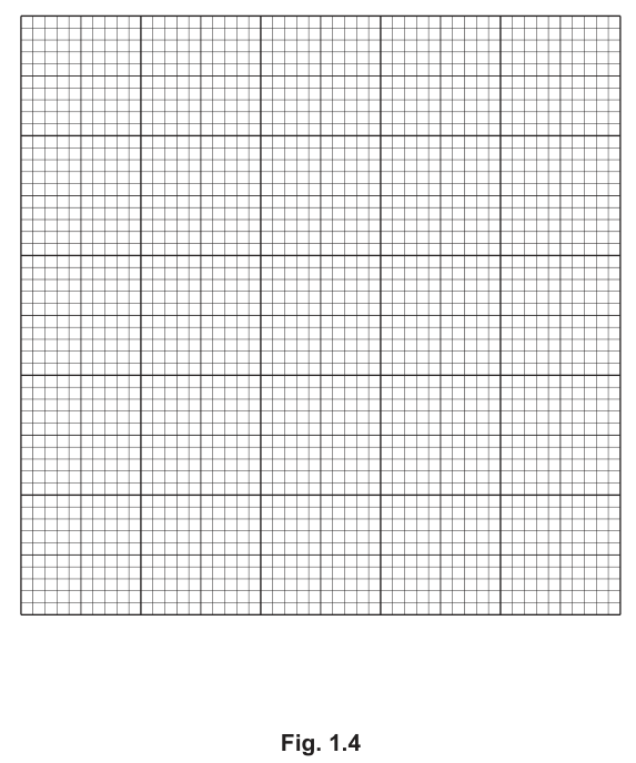
Fig. 1.4
Answer
Plot a bar chart on the grid in Fig. 1.4 with the following features:
- y-axis: 'concentration of sugar / a.u'
- y-axis scale: 5 a.u to 2 cm, origin at zero, with labels at 0, 5, 10, 15 and 20 a.u (every 2 cm)
- x-axis: 'type of fruit juice'
- x-axis: five evenly spaced categories, one for each fruit juice (RG, WG, OR, PA, GF)
- five separate bars of equal width, each with precise horizontal and vertical lines, plotted to the heights given in Table 1.2:
Bar chart with y-axis 'concentration of sugar / a.u' (scale 5 a.u to 2 cm, origin at zero, labelled every 2 cm), x-axis 'type of fruit juice' (five evenly spaced categories), and five bars of equal width at heights 21.25 (RG), 18.50 (WG), 11.75 (OR), 10.25 (PA), 14.00 (GF) a.u.
Background Concept
A bar chart is the appropriate graph for discrete, categorical data (here, five different fruit juices). Each fruit juice is a separate category on the x-axis, and the bar height represents the value of the dependent variable (concentration of sugar) for that category.
For CIE bar charts:
- The y-axis must have a clear scale with the origin at zero (unless there is a good reason to use a broken axis).
- The scale should be chosen so that the bars fill at least half the grid.
- Labels must be placed on the axes (no units in the body of the chart).
- Bars must be of equal width and evenly spaced, with clear horizontal and vertical lines.
- Bars should be drawn with a sharp pencil, using a ruler for the straight edges.
Understanding the Question
Table 1.2 gives the concentration of sugar (in arbitrary units) for five different fruit juices. The candidate must plot this data as a bar chart on the grid in Fig. 1.4.
Approach
- Decide on the y-axis scale: the largest value is 21.25, so a scale of 5 a.u per 2 cm (so 25 a.u fills 10 cm) is appropriate. This fits the grid in Fig. 1.4 (which is about 9 cm tall).
- Label the y-axis with the quantity and the unit (concentration of sugar / a.u).
- Label the x-axis with the categories (type of fruit juice).
- Plot each bar to the correct height, with the fruit juices in any clear order (e.g. the order in Table 1.2: RG, WG, OR, PA, GF).
- Check that all bars are of equal width, evenly spaced, and drawn with precise lines.
Step-by-Step Reasoning
The mark scheme awards four points:
-
Axis labels — y-axis: 'concentration of sugar / a.u' (or equivalent); x-axis: 'type of fruit juice'. Both labels must be present.
-
Scales — y-axis: 5 a.u to 2 cm, labelled at least every 2 cm (so labels at 0, 5, 10, 15, 20), origin at zero. x-axis: even width of bars (all bars the same width, with even gaps between them).
-
Correct plotting — all five bars must be plotted to the correct heights (21.25, 18.50, 11.75, 10.25, 14.00 a.u).
-
Bars drawn precisely — each bar must be a separate rectangle with horizontal and vertical lines joined precisely (no gaps, no overshoots, no slanted lines).
The grid in Fig. 1.4 is approximately 30 small squares wide by 45 small squares tall (each small square = 2 mm). At 5 a.u per 2 cm, each a.u is 2 small squares. So the bar heights in small squares are:
- RG (21.25 a.u) = 42-43 small squares
- WG (18.50 a.u) = 37 small squares
- OR (11.75 a.u) = 23-24 small squares
- PA (10.25 a.u) = 20-21 small squares
- GF (14.00 a.u) = 28 small squares
The y-axis labels are at 0, 10, 20, 30, 40 small squares (= 0, 5, 10, 15, 20 a.u).
Key Takeaways
- Bar charts are used for categorical (discrete) data.
- The y-axis must have a clear scale with the origin at zero.
- Bars must be of equal width, evenly spaced, and drawn precisely.
- CIE bar charts: 5 a.u per 2 cm is a standard scale; the scale should fill at least half the grid.
Common Mistakes
- Using a scale that is too small (e.g. 5 a.u per 1 cm, which would make the bars too short) or too large (e.g. 5 a.u per 5 cm, which would make the bars too tall to fit).
- Not labelling the axes (or labelling them without units).
- Drawing bars of unequal width or with uneven gaps.
- Plotting a bar to the wrong height (e.g. confusing 18.50 with 14.00).
- Using a line graph instead of a bar chart (the data are categorical, not continuous).
- Drawing the bars with slanted or wobbly lines (use a ruler and a sharp pencil).
Things to Be Careful About
- The order of the bars on the x-axis is not specified, but it should be consistent and clear. Using the order in Table 1.2 (RG, WG, OR, PA, GF) is a safe choice.
- The y-axis scale must start at zero; the largest value is 21.25, so the scale must go up to at least 25 a.u.
- The candidate should use a sharp pencil and a ruler; marks are awarded for the precision of the bar drawing.
The rest of this paper
1 more questions- Q2Use of the Light Microscope · Analysis, Conclusions and Evaluation19M