Biology 9700/54 — October/November 2025
Cambridge A-Level · Planning, Analysis and Evaluation · worked solutions for every part, with the mark scheme
Topics Planning · Analysis, Conclusions and Evaluation
Beta vulgaris vulgaris, as shown in Fig. 1.1, is a food crop with a swollen, edible root known as beetroot.
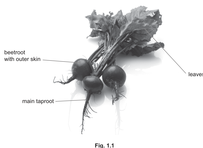
Fig. 1.1
A student determined the concentration of a sucrose solution that has the same water potential as the cells of the beetroot.
The student used distilled water and a stock solution of sucrose to prepare a range of sucrose solutions.
Each sucrose solution was prepared using proportional dilution and had a final volume of .
Complete Table 1.1 to show how the concentrations were made.
Table 1.1
| final concentration of sucrose solution / | volume of distilled water / | volume of stock sucrose solution / |
|---|---|---|
| 2.0 | 0.0 | 30.0 |
| 0.0 | 30.0 | 0.0 |
Answer
For a proportional dilution from a stock to a final volume of :
A representative series (any set of sensible intermediate concentrations is accepted):
| final concentration of sucrose solution / | volume of distilled water / | volume of stock sucrose solution / |
|---|---|---|
| 2.0 | 0.0 | 30.0 |
| 1.5 | 7.5 | 22.5 |
| 1.0 | 15.0 | 15.0 |
| 0.5 | 22.5 | 7.5 |
| 0.25 | 27.5 | 2.5 |
| 0.0 | 30.0 | 0.0 |
See working
Background Concept
A proportional (or serial) dilution is a way of making a range of known concentrations from one stock solution. The rule is that the moles of solute (or stock) needed stay in proportion to the desired final concentration, while the total volume of the solution is held constant.
The general relationship is:
where and are the concentration and volume of the stock solution being drawn up, and and are the desired concentration and the final volume of the diluted solution. Rearranged for the volume of stock required:
Understanding the Question
The student is told the stock sucrose is , the final volume of every working solution is , and the dilution is to be done proportionally (so must always be some simple fraction of ). Table 1.1 has the top row (: no water, stock) and the bottom row (: water, no stock) already filled in; the four blank rows in between need filling.
The mark scheme accepts "any sensible concentrations", so the choice of intermediate values is the candidate's, but they must add up to in every row, and the volumes must be consistent with the chosen concentration.
Approach
- Pick a sensible spread of intermediate concentrations between and (e.g. , , , ). A simple series spaced roughly evenly works well; very large or very small steps risk missing the point where the cells neither gain nor lose mass.
- For each concentration, use the dilution formula to find the volume of stock.
- The volume of distilled water is then .
Step-by-Step Reasoning
Using :
- For : , so water .
- For : , so water .
- For : , so water .
- For : , so water .
In every row the two right-hand volumes must sum to , which acts as a useful consistency check.
Key Takeaways
- A proportional dilution keeps the total volume constant and varies only the ratio of stock to water.
- Use and remember to convert units consistently.
- A wide enough spread of concentrations is needed so that the x-intercept (the cell's water-potential-equivalent concentration) is bracketed.
Common Mistakes
- Using a different final volume (e.g. forgetting that the total must be each time).
- Picking concentrations that cluster at one end of the range, so the answer cannot be interpolated.
- Forgetting to add the correct units on the volumes.
Things to Be Careful About
- The mark scheme accepts any "sensible" set of concentrations, so a different series (e.g. , , , ) scores equally well, provided the volumes are correct.
- Make sure the rows go in order of decreasing concentration, matching the table layout given.
Describe a method the student could use to collect the data needed to determine the concentration of a sucrose solution that has the same water potential as the cells of the beetroot.
The student was supplied with the sucrose solutions prepared in 1(a) and standard laboratory equipment.
Do not include details of how the student:
- prepared the sucrose solutions in 1(a)
- would use the data collected to determine the concentration of a sucrose solution that has the same water potential as the cells of the beetroot.
Your method should be set out in a logical order and be detailed enough to allow another person to follow it.
Answer
- Use beetroots of the same variety and approximately the same age (and from the same batch) to control for biological variation between plants.
- Cut off and discard the outer skin of the beetroot, then use a cork borer (or scalpel and ruler) to cut several cylindrical blocks of equal dimensions (e.g. diameter), cutting onto a white tile with the blade directed away from the hand.
- Label one beaker/container per sucrose concentration (and one for distilled water) and add a known volume (e.g. ) of the appropriate solution to each.
- Blot the cut beetroot blocks dry with filter paper and weigh each block to record the initial mass.
- Place at least three beetroot blocks in each concentration of sucrose solution, ensuring the blocks are fully submerged.
- Leave all the beakers for the same stated time period (e.g. minutes) at room temperature.
- Remove the blocks, blot them dry with filter paper to remove excess surface liquid, and reweigh to obtain the final mass.
- Calculate the percentage change in mass for each block; then calculate the mean percentage change in mass for each sucrose concentration.
- Safety: wear gloves when handling the beetroot (potential irritant/allergen) and cut away from the hand onto a board when using the scalpel/cork borer.
See working
Background Concept
A plant tissue such as beetroot behaves like a partially permeable system. The cell surface membrane and the tonoplast are freely permeable to water but largely impermeable to the solutes inside the vacuole. If the tissue is bathed in a solution whose water potential () is higher (less negative) than that of the cell sap, water enters the cells by osmosis and the tissue gains mass. If of the solution is lower (more negative) than the cell sap, water leaves the cells and the tissue loses mass. At the concentration of sucrose whose matches the cell sap, there is no net movement of water and the mass does not change.
A good experimental method must therefore:
- standardise the tissue (variety, age, dimensions, surface preparation);
- use enough tissue per condition and replicate to get a reliable mean;
- measure mass accurately before and after a fixed exposure time;
- remove surface liquid before weighing (otherwise a wetter block reads artificially heavier);
- control or note safety hazards.
Understanding the Question
Part (b) is an open-ended "describe the method" question worth 7 marks. The student already has the six sucrose solutions from 1(a) plus standard lab equipment. The instructions explicitly exclude two things: how the solutions were prepared (1(a) already covers that) and how the data are used afterwards to estimate the water-potential-equivalent concentration (1(c)(ii) covers that). Everything else belongs in the method.
The mark scheme offers 10 distinct creditable points; the candidate needs 7 of them. The strongest answers thread the points into a logical, ordered procedure rather than a list.
Approach
Build the method in the order a real experimenter would do it: prepare the tissue → standardise the tissue → set up the conditions → measure initial mass → expose for a fixed time → measure final mass (with surface liquid removed) → replicate and mean → safety. Mention at every step which variable is being controlled and why.
Step-by-Step Reasoning
- Same variety/age of beetroot. Different cultivars (and plants of different ages) have different cell sap concentrations, so mixing them would confound the result.
- Remove the outer skin. The skin is a waxy, dead layer that does not behave like the storage tissue and would prevent rapid equilibration of the cells with the solution. Peeling exposes living storage parenchyma.
- Same, stated dimensions of block. Surface-area-to-volume ratio determines the rate of osmosis. Blocks of different sizes would reach equilibrium at different rates and to different extents, giving artefactual differences in mass change.
- Apparatus for cutting equal blocks. A cork borer is the easiest way to cut identical cylinders; a scalpel and ruler/template work too. Cuttings must be of similar shape to give comparable surface area.
- Submerge the blocks in the sucrose solution. A labelled test tube or small beaker is suitable; the block must be fully covered so all surfaces are in contact with the solution. The volume of solution should be enough to swamp any osmotic change in the solution's concentration caused by exchange with the tissue.
- Measure initial AND final mass. Initial mass is needed because percentage change in mass is calculated as . Without an initial mass, percentage change cannot be found.
- After a stated time. Enough time must be allowed for osmotic equilibration (typically – minutes), but the time must be the same for every concentration otherwise the comparison is invalid.
- Remove excess liquid before final weighing. Surface liquid adds to the mass; gently blotting with filter paper (or rolling on a paper towel) gives a true reading of tissue mass.
- At least three blocks per concentration and a mean. Replication reduces the effect of biological variation between blocks and makes the result more reliable. A mean should then be calculated for each concentration.
- Safety comment with hazard + risk + precaution. A complete safety point names a hazard, the specific risk it poses, AND the precaution taken. Beetroot pigment is a potential allergen/irritant → wear gloves. Sharp blades (scalpel, cork borer) can cut → cut onto a board/tile, away from the hand.
Key Takeaways
- A practical method must control biological variables (variety, age, size), procedural variables (time, temperature, surface drying), and replicate to give a mean.
- A safety statement that scores full marks names a specific hazard, the specific risk, and the specific precaution — not vague "be careful".
- All mass comparisons are percentage change, not absolute change, because the starting masses are unlikely to be identical.
Common Mistakes
- Stating only the hazard or only the precaution — both must be present, plus the risk.
- Forgetting to remove surface liquid before the final weighing.
- Not stating the time, or using different times for different concentrations.
- Only using one block per concentration (no replication / no mean).
- Mixing up "remove the outer skin" with "cut the beetroot into blocks of equal size" — these are two separate controlled variables in the mark scheme and both earn marks.
Things to Be Careful About
- The question says "standard laboratory equipment" — so apparatus is restricted to the usual lab items (cork borer, scalpel, ruler, beakers, top-pan balance, filter paper, timer). No specialist kit.
- The method should be written as a sequence another person could follow, not as a list of variables.
The student calculated the mean percentage change in mass of the beetroot for each concentration of sucrose solution.
The student plotted these calculated values to obtain a line graph.
Complete Fig. 1.2 by:
- labelling the axes
- sketching the line that the student obtained.
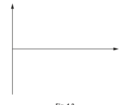
Fig. 1.2
Answer
- x-axis: concentration of sucrose solution / , with the scale running from to .
- y-axis: mean percentage change in mass of beetroot / , with a clear zero line and positive values above and negative values below.
- Sketch: a straight (or near-straight) line sloping downwards from left to right, starting in the positive region of the y-axis at low sucrose concentration and ending in the negative region at high sucrose concentration, crossing the x-axis between and .
See working
Background Concept
The independent variable in this experiment is the concentration of the sucrose solution (varied across the range prepared in 1(a)). The dependent variable is the mean percentage change in mass of the beetroot blocks. The relationship is roughly linear in the practical range:
- In very dilute sucrose (or distilled water), , so water enters the cells, turgor increases and the tissue gains mass (positive percentage change).
- In very concentrated sucrose, , so water leaves the cells, plasmolysis occurs and the tissue loses mass (negative percentage change).
- At the concentration where the solution's equals the cell sap's , there is no net water movement and the percentage change in mass is zero.
The point where the line crosses the x-axis is therefore the answer to the investigation: the concentration of sucrose solution with the same water potential as the beetroot cells.
Understanding the Question
Part (c)(i) supplies a blank graph in Fig. 1.2. The y-axis already has a zero-line drawn (positive above, negative below); the x-axis arrow points to the right. The candidate must label the axes with the correct quantity and unit AND sketch the expected line of best fit.
The mark scheme awards one mark for correctly labelling both axes (with units) and one mark for a sketch that decreases (downward slope) and crosses the x-axis (i.e. passes through the y = 0 line within the plotted range).
Approach
- Decide which variable goes on which axis. Convention: independent variable on the x-axis, dependent on the y-axis.
- Label each axis with the quantity AND the unit (mol dm⁻³ on x; % on y).
- Sketch the expected shape: a downward-sloping line that crosses zero on the y-axis (which is the x-axis intercept).
Step-by-Step Reasoning
- x-axis label: "concentration of sucrose solution / ". The scale should run from at the origin to at the right-hand end, with intermediate marks.
- y-axis label: "mean percentage change in mass of beetroot / %".
- Sketch shape: start in the upper-left (positive percentage change at low sucrose concentration), end in the lower-right (negative percentage change at high sucrose concentration). The line must pass through the y = 0 axis at some x-value between and . A straight line of best fit is appropriate if the data look linear; a gentle curve is acceptable provided the trend is clearly downward.
Key Takeaways
- Axis labels must include both the quantity (what is being plotted) and the unit.
- The trend line in this kind of osmosis experiment is monotonic and crosses the x-axis — that crossing point is the answer to the question.
- A line that only descends but never reaches or crosses the x-axis, or that ascends, fails to score the second mark.
Common Mistakes
- Swapping the axes (e.g. putting concentration on the y-axis).
- Omitting units on the axis labels.
- Drawing a line that is horizontal, or that goes up, or that stays entirely on one side of the x-axis.
- Forgetting that the y-axis has both positive and negative regions — the y = 0 line is the x-axis itself.
Things to Be Careful About
- A "sketch" should be smooth and continuous, not a series of dots-to-dots; the candidate is showing the trend, not individual data points (which would not be visible on a single sketch grid anyway).
Explain how the student used the completed line graph in Fig. 1.2 to estimate the concentration of sucrose solution that has the same water potential as the cells of the beetroot.
Answer
Read the concentration value on the x-axis at the point where the line of best fit crosses the x-axis (i.e. where the mean percentage change in mass = ). This concentration is the one whose water potential equals that of the beetroot cells.
See working
Background Concept
The line drawn in 1(c)(i) summarises the relationship between sucrose concentration and the change in mass of the beetroot tissue. The y-value tells us whether the cells are gaining or losing water; the y = 0 line is the special point at which there is no net movement of water. Because the cells neither gain nor lose water at this concentration, the water potential of the surrounding solution must equal the water potential of the cell sap (the cell is in equilibrium with its surroundings).
Understanding the Question
The question asks the student to explain how the graph is used to estimate the concentration of sucrose whose water potential matches the beetroot cells. It is a one-mark question and the mark scheme credits either of two equivalent statements: identifying the x-axis intercept, OR identifying the point on the x-axis where the percentage change in mass is zero.
Approach
Trace the line of best fit until it crosses the x-axis (the y = 0 line), then drop a vertical line down to the x-axis to read off the corresponding sucrose concentration.
Step-by-Step Reasoning
- Locate the point on the line where it intersects the x-axis. At this point the y-value (percentage change in mass) is exactly zero.
- Read the corresponding x-value. This is the sucrose concentration in .
- This concentration corresponds to a sucrose solution whose water potential equals the water potential of the beetroot cell sap, because there is no net osmotic movement of water in either direction.
Key Takeaways
- The x-intercept of a percentage-change-in-mass vs concentration graph is the water-potential-equivalent concentration.
- The biological reason is that at zero mass change, the cell is in osmotic equilibrium with the external solution.
Common Mistakes
- Reading off the y-intercept (which would correspond to mass change in pure water, not the water-potential-equivalent point).
- Trying to read the answer at the maximum or minimum of the curve instead of the x-intercept.
- Saying "where the line crosses the y-axis" by mistake.
Things to Be Careful About
- The question says "estimate" — the answer is read from a sketch and so is approximate. Quote the concentration to a sensible precision (e.g. one or two significant figures) consistent with the scale of the x-axis.
The cells of the beetroot contain a red pigment which can leak out into the solution when the tissue is cut. The student noticed that each sucrose solution was coloured red at the end of the investigation.
Suggest one improvement the student could make to the method to reduce the amount of red pigment in each sucrose solution.
Answer
Rinse the cut beetroot blocks with distilled water (blot them dry) before placing them into the sucrose solutions, so that any red pigment released during cutting is washed away first and does not contaminate the working solutions.
Rinse the cut beetroot blocks with distilled water before immersing them in the sucrose solutions.
Background Concept
The red-purple colour of beetroot comes from betalain pigments stored in the vacuole of the storage parenchyma cells. The tonoplast and cell surface membrane normally keep these pigments inside the cell, but cutting the tissue damages some cells and ruptures their membranes, releasing the pigment into the surrounding solution. Once in the solution, the pigment has no effect on the mass of the tissue, but it does colour the solution and can stain the apparatus, and any later use of these solutions (e.g. for absorbance work) would be compromised.
The improvement is therefore a step that removes the pigment released by the act of cutting before the experimental exposure begins.
Understanding the Question
The student noticed that all of the sucrose solutions were coloured red at the end of the investigation. The question asks for ONE improvement that would reduce the amount of pigment in the solutions. The mark scheme credits a single point: "rinse (beetroot) blocks (after cutting / before adding to sucrose solution)".
Approach
Identify the source of the pigment (cut cells at the tissue surface) and target that source with a simple pre-treatment step.
Step-by-Step Reasoning
- The pigment leaks out because cutting the beetroot breaks open some cells at the cut surface. The volume of solution is small ( per beaker) so even a small amount of leakage is visible.
- After cutting the blocks, swishing them briefly in distilled water (or rinsing under a wash bottle) removes the pigment already in the damaged surface cells before the block is added to the experimental solution.
- Pat the blocks dry on filter paper before weighing/immersing, so the rinse water does not dilute the sucrose solution or alter the starting mass.
- This is a cheap, low-risk, one-step improvement that directly addresses the source of the contamination.
Key Takeaways
- Limitations can often be fixed by a small change in sample preparation that targets the specific source of the artefact.
- Improvements must be practical, low-risk, and specific to the named limitation — "be more careful" or "use cleaner equipment" would not score.
Common Mistakes
- Suggesting vague improvements like "use a sharper knife" or "be more careful" — these don't specifically remove the pigment that has already leaked from cut cells.
- Suggesting changes that would invalidate the experiment, e.g. using a different tissue.
- Adding detergent or bleach, which would destroy cell membranes and ruin the osmosis experiment.
Things to Be Careful About
- The improvement must reduce the pigment in the SOLUTION, not the tissue; the question is specific about what is to be improved.
- The mark scheme wording is "rinse" — accept synonyms such as "wash".
The buff-tailed bumblebee, Bombus terrestris, is an insect that uses its tongue to feed on the nectar and pollen of flowers.
Buff-tailed bumblebees can feed on the nectar and pollen of flowers by either gripping (holding) onto flower petals or by hovering (flying) in front of the flowers.
Fig. 2.1 shows the buff-tailed bumblebee.
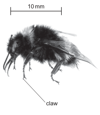
Fig. 2.1
The buff-tailed bumblebee has adaptations, such as claws, to help it to grip on to flower petals to obtain nectar and pollen.
Fig. 2.2 shows the buff-tailed bumblebee using its claws to grip on to the flower petals as the bee feeds.
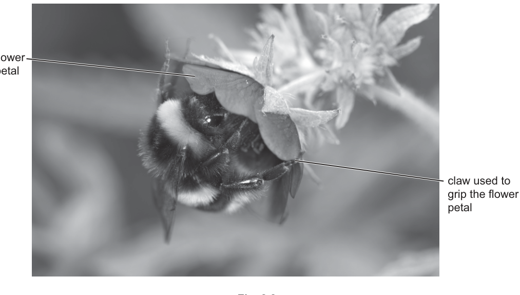
Fig. 2.2
Fig. 2.3 is a magnified image of the claw of a bee.
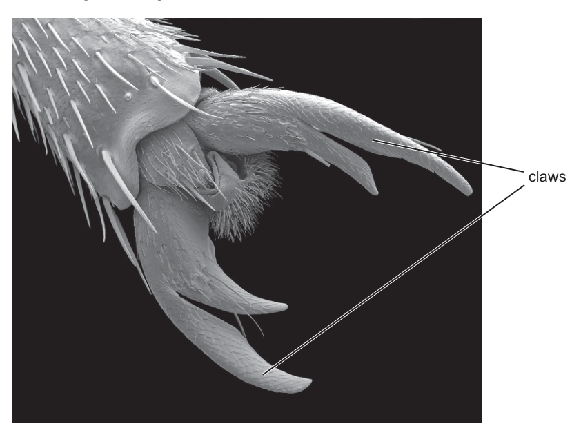
Fig. 2.3
Suggest a method that can be used to measure the image length of the longest part of the curved claw in Fig. 2.3.
Answer
Lay a piece of thread (or cotton/string) along the curved outline of the claw, mark the two end points on the thread, then straighten the thread and measure its length against a ruler.
Use thread to trace the curve, mark the ends, straighten and measure against a ruler.
Background Concept
When measuring lengths on a printed image or photograph, a standard ruler can only accurately measure straight lines. Curved structures (such as the curved claw in Fig. 2.3) cannot be measured directly with a ruler because the ruler is rigid and straight. To measure a curved length, a flexible medium is required that can be laid along the curve, then straightened and measured against a ruler.
Understanding the Question
Fig. 2.3 is a scanning electron micrograph of a bee's foot, showing two curved, pointed claws. The question asks for a method to measure the image length of the longest part of the curved claw. This is a single-mark question testing whether the candidate knows the standard practical technique for measuring curved lines on an image.
Approach
Use a non-rigid, flexible material (such as thread, cotton, or string) to trace the curve, then straighten it and measure with a ruler. This is the standard method in biology practical work for measuring curved or irregular lengths on printed images.
Step-by-Step Reasoning
- The claw in Fig. 2.3 is clearly curved, so a direct ruler measurement would be inaccurate.
- A flexible medium (thread, cotton, or string) can be laid along the curve to follow its contour exactly.
- Once the thread has been laid along the curve, mark the position of the two ends of the claw on the thread.
- Remove the thread, lay it flat against a ruler, and read off the distance between the two marks.
- This gives the image length of the curved claw.
Key Takeaways
- Curved lines on images are measured by tracing with a flexible medium, then straightening and measuring against a ruler.
- This is a general practical skill applicable to many measurements in biology (e.g., measuring curved roots, leaves, or organisms on photographs).
Common Mistakes
- Suggesting using a ruler alone (cannot measure curves accurately).
- Suggesting using a flexible ruler (these are not standard lab equipment and would still be difficult to align with a curve).
- Forgetting to mark the endpoints before straightening the thread.
Things to Be Careful About
- The question asks for a 'method' — describe a procedure, not just state a result.
- The flexible medium should ideally be non-stretchy (cotton or string is more reliable than elastic).
The surfaces of flower petals of different plant species have different textures.
Fig. 2.4 shows a scanning electron micrograph of a rough surface of a flower petal.
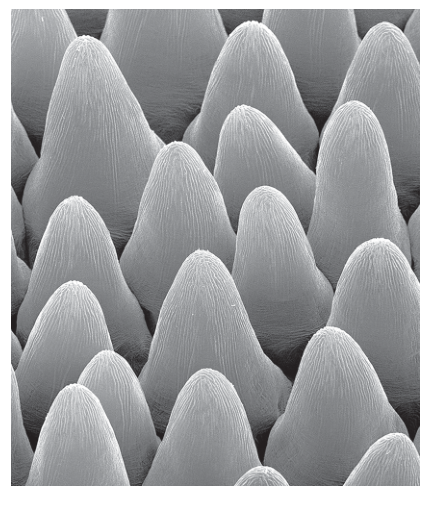
Fig. 2.4
Fig. 2.5 shows a scanning electron micrograph of a smoother surface of a flower petal.
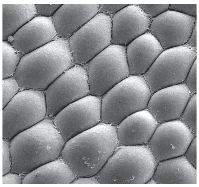
Fig. 2.5
A scientist made an artificial flower apparatus, as shown in Fig. 2.6.
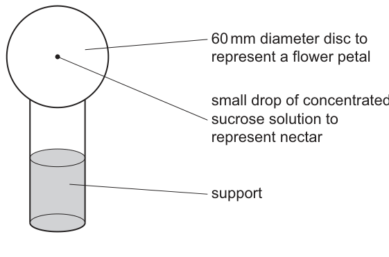
Fig. 2.6
To model flower petals with different levels of roughness, the scientist used different discs.
Each disc was made using particles of different diameters attached to the surface of the disc, as shown in Table 2.1.
Table 2.1
| mean particle diameter on the disc / | level of roughness |
|---|---|
| 5 | smooth |
| 9 | |
| 12 | |
| 16 | |
| 30 | |
| 53 | rough |
The diameter of each disc was standardised as .
Identify one other variable the scientist should standardise when making the discs.
Answer
Any one from:
- colour of the disc
- material the disc is made of
- type (shape) of particle (used to make the disc surface)
e.g. colour of disc / material of disc / type of particle
Background Concept
In a controlled experiment, the independent variable (IV) is deliberately changed by the experimenter, while the dependent variable (DV) is measured. All other variables — called controlled variables (CVs) or standardised variables — must be kept constant to ensure a fair test. If CVs vary, the experimenter cannot be sure that any change in the DV is due to the IV.
Understanding the Question
The scientist is investigating whether the level of roughness of the disc affects whether bees grip or hover. The IV is the level of roughness (i.e., particle diameter). The diameter of the disc (60 mm) has already been standardised. The question asks for ONE other variable that should also be standardised to ensure a fair test.
Approach
Think about what else could differ between the discs that might also affect whether the bee grips or hovers. The mark scheme accepts three specific answers: colour of the disc, material the disc is made of, or type (shape) of particle. Any of these is a valid answer.
Step-by-Step Reasoning
- The IV is the particle diameter (which determines the level of roughness).
- To make this a fair test, every other factor that might affect whether the bee grips or hovers must be kept the same across all discs.
- Valid standardised variables include:
- Colour of the disc — bees see colour and might be influenced by it; if discs were different colours, the bee's response could be due to colour rather than roughness.
- Material the disc is made of — different materials might have different grip properties beyond just the particle coating.
- Type (shape) of particle — if particle shapes differ between discs, this could change grip independently of particle diameter.
- Any one of these would earn the mark.
Key Takeaways
- Standardised (controlled) variables are those kept constant in a fair test.
- The mark scheme gives three possible answers; any one is acceptable.
Common Mistakes
- Saying 'particle diameter' — this IS the independent variable, not a controlled variable.
- Saying 'the bees' or 'the same bees' — although using the same colony might be a control, the question specifically asks about variables relating to the discs.
- Giving vague answers like 'temperature' or 'time' without a clear link to the experimental setup.
Things to Be Careful About
- The question says 'one other variable' — only one is needed, but any single valid answer will earn the mark.
- The mark scheme is specific: colour, material, or type of particle. Other plausible answers (e.g., concentration of sucrose, time of day) might be considered but are not on the mark scheme.
The scientist investigated if the level of roughness of the discs affects whether buff-tailed bumblebees grip on to the disc or hover when they feed (feeding visit) from the small drop of concentrated sucrose solution.
For each disc, the scientist:
- recorded the number of feeding visits when the buff-tailed bumblebees gripped on to the disc
- recorded the number of feeding visits when the buff-tailed bumblebees hovered in front of the disc
- calculated the percentage of feeding visits when the buff-tailed bumblebees gripped on to the disc.
State the independent variable in this investigation.
Answer
The independent variable is the (mean) particle diameter on the disc / (level of) roughness of the disc.
(mean) particle diameter on the disc (or level of roughness)
Background Concept
In any experiment, the independent variable (IV) is the variable that the experimenter deliberately changes. It is what the experimenter manipulates to test its effect on the dependent variable (DV), which is the variable that is measured.
Understanding the Question
The scientist has made discs with different particle diameters to model different levels of roughness. For each disc, the percentage of feeding visits when bees gripped is calculated. The IV is the variable the scientist is changing between trials.
Approach
Identify what is different between the discs: the mean particle diameter. The mark scheme accepts either '(level of) roughness' or '(mean) particle diameter (on disc)' — these are two ways of describing the same underlying variable.
Step-by-Step Reasoning
- The scientist has six discs, each with a different mean particle diameter (5, 9, 12, 16, 30, 53 µm).
- These different particle diameters correspond to different levels of roughness (Table 2.1 marks 5 µm as 'smooth' and 53 µm as 'rough').
- This is what is being deliberately changed between trials, so it is the independent variable.
- The dependent variable is the percentage of feeding visits when the bees gripped (or, equivalently, hovered).
Key Takeaways
- The IV is what the experimenter varies.
- Either 'particle diameter' or 'level of roughness' is a correct answer; they describe the same underlying variable.
Common Mistakes
- Stating the DV (percentage of feeding visits when bees gripped) instead of the IV.
- Stating a controlled variable (e.g., disc diameter) instead of the IV.
- Confusing the IV with the experimental apparatus (e.g., saying 'the disc' rather than what differs between discs).
Things to Be Careful About
- The mark scheme accepts either wording; both refer to the same underlying variable.
For the disc with a mean particle diameter of , the scientist calculated that the buff-tailed bumblebees gripped on to the disc for of their feeding visits.
The total number of feeding visits was .
Calculate the number of feeding visits when the buff-tailed bumblebees hovered in front of the disc.
Give your answer to the nearest whole number.
number of feeding visits when the buff-tailed bumblebees hovered = ______
Working
% of visits when hovering = 100 − 79 = 21%
Number of visits when hovering = (21 / 100) × 117 = 24.57
Answer
25 (or 24) feeding visits
25 (or 24)
Background Concept
Percentages represent parts of a whole. If a percentage of events are of one type, the remaining percentage must be of the other type. To convert a percentage to a count, multiply the total by the percentage (as a decimal).
Understanding the Question
For the 16 µm disc, 79% of the 117 feeding visits involved the bee gripping on to the disc. We need to calculate how many visits involved the bee hovering. Since every visit is either 'grip' or 'hover', the percentages of grip and hover must sum to 100%.
Approach
Subtract the grip percentage from 100% to get the hover percentage, then multiply by the total number of visits.
Step-by-Step Reasoning
- % hover = 100 − 79 = 21%
- Number hovering = (21/100) × 117 = 24.57
- Rounded to the nearest whole number = 25 (since 24.57 is closer to 25 than to 24).
- The mark scheme accepts either 24 or 25 (this is generous rounding: 24.57 strictly rounds to 25, but the mark scheme permits 24 to allow for candidates who truncate or who use a slightly different intermediate step).
Key Takeaways
- Percentages of two complementary categories must sum to 100%.
- Always round to the precision requested (here, nearest whole number).
- The number of visits must be a whole number (you cannot have a fraction of a visit).
Common Mistakes
- Subtracting 79 from 117 directly (this gives 38, which is the number of grip visits, not hover).
- Forgetting to round to the nearest whole number.
- Confusing 'gripping visits' with 'hovering visits' and accidentally using 79% instead of 21%.
Things to Be Careful About
- The answer is a whole number of visits.
- The mark scheme accepts both 24 and 25 — but the more mathematically correct answer (to the nearest whole number) is 25.
Fig. 2.7 shows the results of the investigation.
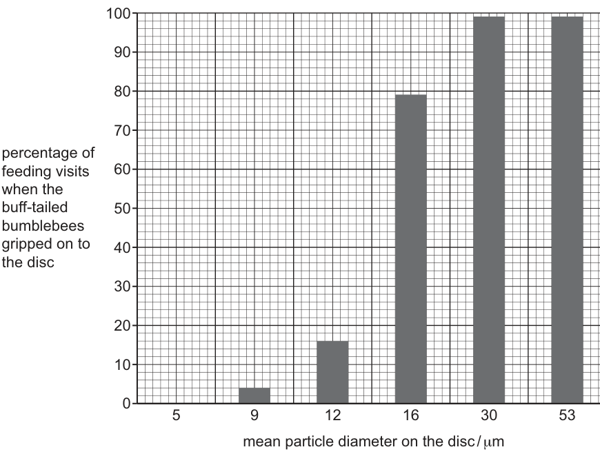
Fig. 2.7
State two conclusions that can be made from the results in Fig. 2.7.
Answer
Any two from:
- As the (mean) particle diameter on the disc increases, the percentage of feeding visits when the bees gripped on to the disc increases (ora: as particle diameter decreases, the percentage gripping decreases).
- At 30 µm and 53 µm (above 30 µm), there is no further increase / no change in the percentage of feeding visits when the bees gripped on to the disc.
- At 5 µm, the bees only hovered (0% of visits involved gripping).
Two valid conclusions from the bar chart (trend, plateau at high values, or minimum at 5 µm)
Background Concept
Conclusions drawn from a bar chart should be based on specific trends, values, and patterns in the data. A good conclusion:
- Describes the overall trend (using the variables on the axes).
- Mentions specific values or features (e.g., maxima, minima, plateaus, anomalies).
- Uses precise language tied to the data shown.
Understanding the Question
Fig. 2.7 is a bar chart showing the percentage of feeding visits when bees gripped against the mean particle diameter. The data are: 5 µm = 0%, 9 µm ≈ 4%, 12 µm ≈ 16%, 16 µm ≈ 79%, 30 µm ≈ 99%, 53 µm ≈ 99%. The question asks for two conclusions from this data.
Approach
Identify the overall trend, then identify specific features (plateaus, end points, anomalies). Any two of these earn 2 marks.
Step-by-Step Reasoning
- The overall trend: as particle diameter increases from 5 to 30 µm, the percentage of gripping increases (from 0% to ~99%). This is a positive correlation.
- Plateau: at 30 µm and 53 µm, the values are both ~99% — there is no further increase above 30 µm.
- Specific point: at 5 µm (the smallest particle diameter), 0% of visits involved gripping — the bees only hovered.
- Any two of these conclusions earn 2 marks.
Key Takeaways
- Read the overall trend (positive correlation between particle diameter and % gripping).
- Read the plateau (no change above 30 µm — the relationship is not linear throughout).
- Read the minimum (0% at 5 µm — bees only hover on the smoothest surface).
- Each conclusion should be supported by the data shown.
Common Mistakes
- Saying 'gripping increases' without specifying with what (it should be with particle diameter).
- Vague descriptions like 'the bees prefer rough surfaces' — this over-generalises and is not directly supported by the data shown.
- Saying 'bees always grip on rough surfaces' — this is too absolute; even at 53 µm, only ~99% gripped, not 100%.
- Failing to mention a specific value or feature from the chart.
Things to Be Careful About
- Use the language of the question (mean particle diameter, percentage of feeding visits, gripped on to the disc).
- The data end at 53 µm — we cannot conclude anything about particle diameters above this.
- The trend is non-linear: there is a rapid increase between 12 and 30 µm, then a plateau.
A student used the Spearman’s rank correlation to analyse the data in Fig. 2.7.
The student stated the null hypothesis as:
There is no correlation between the mean particle diameter on the disc and the percentage of feeding visits when the buff-tailed bumblebees gripped on to the disc.
The formula for Spearman’s rank correlation () is:
key to symbols:
= difference in rank between each pair of measurements
= number of pairs of items in the sample
Complete Table 2.2 to calculate .
Table 2.2
| mean particle diameter on the disc / | rank of mean particle diameter on the disc | percentage of feeding visits when the buff-tailed bumblebees gripped on to the disc | rank of percentage of feeding visits when the buff-tailed bumblebees gripped on to the disc | Difference in rank, | |
|---|---|---|---|---|---|
| 5 | 1 | 0 | |||
| 9 | 2 | 4 | |||
| 12 | 3 | 16 | |||
| 16 | 4 | 79 | |||
| 30 | 5 | 99 | |||
| 53 | 6 | 99 | |||
Answer
| mean particle diameter on the disc / µm | rank of mean particle diameter on the disc | percentage of feeding visits when the buff-tailed bumblebees gripped on to the disc | rank of percentage of feeding visits when the buff-tailed bumblebees gripped on to the disc | Difference in rank, | |
|---|---|---|---|---|---|
| 5 | 1 | 0 | 1 | 0 | 0 |
| 9 | 2 | 4 | 2 | 0 | 0 |
| 12 | 3 | 16 | 3 | 0 | 0 |
| 16 | 4 | 79 | 4 | 0 | 0 |
| 30 | 5 | 99 | 5.5 | 0.5 | 0.25 |
| 53 | 6 | 99 | 5.5 | 0.5 | 0.25 |
| 0.5 |
ΣD² = 0.5
Background Concept
Spearman's rank correlation coefficient () measures the strength and direction of a monotonic relationship between two variables. The first step is to rank both variables (lowest = rank 1, highest = rank ). When two values are tied, they share a rank equal to the mean of their position ranks.
Understanding the Question
The table gives the raw data (mean particle diameter and % of gripping). The first column (rank of mean particle diameter) is already completed. The candidate must rank the second variable (% of gripping), find the difference in rank () for each pair, square the differences, and sum them to get .
Approach
- Rank the % of gripping (0%, 4%, 16%, 79%, 99%, 99%).
- Find for each pair (the difference between the two ranks).
- Square each .
- Sum the squared values.
Step-by-Step Reasoning
- Particle diameter ranks are given: 5=1, 9=2, 12=3, 16=4, 30=5, 53=6.
- % of gripping ranks:
- 0% is the lowest → rank 1
- 4% → rank 2
- 16% → rank 3
- 79% → rank 4
- 99% appears twice (at 30 and 53 µm). The two position ranks are 5 and 6, so the mean rank is (5+6)/2 = 5.5. Both values get rank 5.5.
- Differences in rank ():
- 5 µm: 1 − 1 = 0
- 9 µm: 2 − 2 = 0
- 12 µm: 3 − 3 = 0
- 16 µm: 4 − 4 = 0
- 30 µm: 5 − 5.5 = −0.5 (use absolute value for )
- 53 µm: 6 − 5.5 = 0.5
- values: 0, 0, 0, 0, 0.25, 0.25
Key Takeaways
- Tied values get the mean of their position ranks (not the lower or upper rank).
- is the difference in rank, and the sign does not matter for .
- is then used in the Spearman's rank formula.
Common Mistakes
- Giving tied values different ranks (e.g., 5 and 6 instead of 5.5 and 5.5) — this would change .
- Forgetting to square the differences.
- Adding the differences directly instead of the squared differences.
Things to Be Careful About
- Always check for tied values before ranking. The mark scheme specifically requires the tied ranks of 5.5.
- The formula uses (squared), so the negative sign for at 30 µm does not affect the final answer.
Working
,
Answer
(or 0.986 to 3 d.p.)
0.99 (or 0.986)
Background Concept
Spearman's rank correlation coefficient is calculated using the formula:
where is the number of pairs and is the sum of squared rank differences. The value of ranges from (perfect negative correlation) through 0 (no correlation) to (perfect positive correlation).
Understanding the Question
The candidate must use the value of from part (c)(i) and to calculate .
Approach
Substitute the values into the formula and evaluate step by step. Show the working clearly so that the calculation can be followed.
Step-by-Step Reasoning
- ,
- Calculate :
- Calculate :
- Calculate the fraction: (to 5 d.p.)
- Subtract from 1:
- Rounded to 2 d.p.: 0.99; to 3 d.p.: 0.986.
Key Takeaways
- The Spearman's rank formula is a standard statistical calculation.
- indicates a very strong positive correlation between the mean particle diameter and the % of gripping.
- The mark scheme accepts 0.99 (to 2 d.p.) or 0.986 (to 3 d.p.).
Common Mistakes
- Calculating incorrectly (e.g., as instead of ).
- Forgetting the negative sign in the formula.
- Using 0.5 as the numerator instead of .
- Failing to round the answer.
Things to Be Careful About
- The order of operations matters: calculate first, then divide by , then subtract from 1.
- The mark scheme accepts 0.99 or 0.986 — both are correct to different numbers of decimal places.
Table 2.3 shows the critical values of at the probability level.
Table 2.3
| 5 | 6 | 7 | 8 | 9 | 10 | 11 | 12 | |
|---|---|---|---|---|---|---|---|---|
| critical value of | 0.90 | 0.83 | 0.71 | 0.64 | 0.60 | 0.56 | 0.54 | 0.50 |
Use the data from Table 2.3 to explain why the student rejected the null hypothesis.
Answer
At , the critical value of at the 0.05 probability level is 0.83 (from Table 2.3). The calculated value of (0.99) is greater than this critical value, so there is a significant correlation between the mean particle diameter on the disc and the percentage of feeding visits when the bees gripped on to the disc, and the null hypothesis is rejected.
calculated rs (0.99) > critical value (0.83) at n=6, p=0.05, so reject the null hypothesis
Background Concept
The Spearman's rank correlation coefficient is interpreted by comparing the calculated value to a critical value at a chosen significance level (usually 0.05 or 5%). If the calculated value is greater than the critical value (in absolute terms), the null hypothesis is rejected — meaning there is a statistically significant correlation between the two variables.
Understanding the Question
The calculated (or 0.986). For , the critical value of at the 0.05 probability level is 0.83 (from Table 2.3). The student rejected the null hypothesis. The question asks for the explanation of why the null hypothesis was rejected.
Approach
Compare the calculated to the critical value, and state which is greater. State the conclusion in terms of the null hypothesis.
Step-by-Step Reasoning
- The calculated (or 0.986).
- From Table 2.3, at , the critical value at is 0.83.
- The calculated (0.99) is greater than the critical value (0.83).
- This means the correlation is statistically significant at the 0.05 level (the probability of getting this correlation by chance, if the null hypothesis were true, is less than 5%).
- Therefore, the null hypothesis (no correlation) is rejected.
Key Takeaways
- A calculated test statistic greater than the critical value leads to rejection of the null hypothesis.
- Statistical significance is at the chosen probability level (here, 0.05 or 5%).
- The conclusion is that there is a significant positive correlation between the mean particle diameter and the % of gripping visits.
Common Mistakes
- Saying ' is less than 0.83' — this would mean failing to reject the null hypothesis, which is wrong here.
- Not mentioning the critical value from the table.
- Not referring to the calculated value.
- Saying the correlation is negative (it is positive, as is close to +1).
Things to Be Careful About
- The critical value depends on both and the probability level.
- At , , the critical value is 0.83.
- The conclusion is that the correlation between particle diameter and % gripping is significant — this is consistent with the visual trend in Fig. 2.7.
Pectin is a polysaccharide found in plant cell walls. Pectinase is an enzyme that hydrolyses pectin.
A student investigated the use of pectinase to extract more juice from different types of fruit.
The student:
- removed the outer skin and cut each type of fruit into small pieces
- placed each type of fruit into a separate beaker with of pectinase solution
- incubated the mixture at for minutes
- passed the contents of the beaker through a filter funnel into a measuring cylinder
- measured the volume of juice extracted from each type of fruit.
Table 3.1 shows the results.
Table 3.1
| type of fruit | volume of juice extracted / | |||
|---|---|---|---|---|
| sample 1 | sample 2 | sample 3 | mean of samples | |
| apple | 16 | 17 | 17 | |
| orange | 30 | 37 | 33 | |
| pineapple | 41 | 44 | 45 | |
| grapes | 17 | 15 | 11 |
Working
- Apple:
- Orange:
- Pineapple:
- Grapes:
Answer
| type of fruit | mean of samples / |
|---|---|
| apple | 16.7 |
| orange | 33.3 |
| pineapple | 43.3 |
| grapes | 14.3 |
apple 16.7, orange 33.3, pineapple 43.3, grapes 14.3 cm³
Background Concept
When a measurement is repeated, individual values vary due to random error and uncontrolled factors. The arithmetic mean of the repeated values is the best estimate of the true value because positive and negative deviations from the true value tend to cancel out. For repeated measurements, the mean is the sum of the values divided by . The mean is usually recorded to one decimal place beyond the precision of the original data, or to the same precision if the result happens to be exact.
Understanding the Question
The student repeated the juice-extraction experiment three times for each of four fruit types and recorded the volume of juice in cm³ in Table 3.1. The 'mean of samples' column is blank. The task is to calculate the mean volume for each fruit and write it into the table.
Approach
For each row, add the three sample values and divide by 3. The answer should be quoted in cm³ to one decimal place (since three values rarely sum to a multiple of 3).
Step-by-Step Reasoning
- Apple: , then cm³ → record as cm³ (or cm³ if rounded to the nearest whole number).
- Orange: , then cm³ → cm³.
- Pineapple: , then cm³ → cm³.
- Grapes: , then cm³ → cm³.
Each mean lies between the smallest and largest sample value in its row, which is a quick sanity check that the calculation is correct.
Key Takeaways
- The mean of repeated measurements is the standard way to summarise and reduce the effect of random error.
- Round the mean to a sensible number of decimal places — here, one decimal place is appropriate.
- The mean should lie between the minimum and maximum of the sample values; if it does not, the calculation has an error.
Common Mistakes
- Rounding each sample before adding (this introduces extra rounding error and is unnecessary).
- Forgetting to record the units (cm³).
- Dividing by the wrong number (e.g., 2 instead of 3).
- Mixing up the rows when transferring the answer to the table.
Things to Be Careful About
- The mark scheme accepts whole-number means () when three values sum to a multiple of 3, but since none of these rows sum exactly to a multiple of 3, the one-decimal-place form () is the more accurate answer.
- The same unit (cm³) should be used in the working and the table.
The independent variable is the type of fruit and the dependent variable is the volume of juice extracted.
Complete Table 3.2 to show the type of variable and the type of data.
Table 3.2
| type of variable | type of data | |
|---|---|---|
| type of fruit | ||
| volume of juice extracted |
Answer
Table 3.2 completed:
| type of variable | type of data | |
|---|---|---|
| type of fruit | categoric / qualitative | nominal |
| volume of juice extracted | quantitative | continuous |
type of fruit — categoric / qualitative, nominal; volume of juice extracted — quantitative, continuous
Background Concept
Variables in an experiment can be classified in two complementary ways.
Type of variable:
- Categoric (qualitative): a variable that places each item into one of several named categories with no inherent numerical order (e.g., apple, orange, pineapple, grapes).
- Quantitative: a variable that takes numerical values.
Type of data:
- Nominal: data consisting of named categories with no order.
- Ordinal: data consisting of named categories that can be ranked (e.g., small, medium, large).
- Discrete: numerical data that can only take specific separate values (usually whole-number counts).
- Continuous: numerical data that can take any value within a range, including fractions and decimals.
These classifications determine which statistical tests and graphical displays are appropriate: nominal data are summarised as percentages or mode; ordinal as median or mode; continuous data as mean and standard deviation.
Understanding the Question
Two variables are given: the independent variable (type of fruit) and the dependent variable (volume of juice extracted). The task is to identify, for each, the type of variable and the type of data, and write these into Table 3.2.
Approach
For each variable, apply the two classifications:
- A variable that is a named group with no numerical value is categoric / qualitative, and the data are nominal.
- A variable measured on a numerical scale (where the measurement can fall anywhere on a continuous range) is quantitative and the data are continuous.
Step-by-Step Reasoning
- Type of fruit: the four fruit types are distinct named categories with no inherent numerical order (apple is not 'less than' orange). It is therefore a categoric variable, and the data are nominal.
- Volume of juice extracted: measured in cm³ using a measuring cylinder, which can read to any value on the continuous scale (e.g., 33.3 cm³). It is therefore a quantitative variable, and the data are continuous.
Key Takeaways
- Categoric variables are names with no numbers; quantitative variables are numbers.
- Nominal data are names with no order; continuous data are numbers on a continuous scale.
- A volume measurement with a graduated cylinder is continuous; a count of items is discrete.
Common Mistakes
- Writing 'independent/dependent' or 'controlled variable' — these describe the role of the variable in the experiment, not the type.
- Describing volume as 'discrete' because the recorded values happen to be integers — the underlying scale is continuous.
- Confusing ordinal (ranked categories) with nominal (unranked categories).
Things to Be Careful About
- The mark scheme accepts 'qualitative' as equivalent to 'categoric'; either word scores the mark.
- 'Continuous' applies because the measuring cylinder can in principle read to any value; the fact that the student's readings happen to be whole numbers does not change the type of data.
State two changes the student should make to their method to improve the quality of their results.
Answer
- Standardise the total mass / volume / number / size of (each) fruit piece used;
- Use fruit of the same age / ripeness for each type of fruit.
(Other acceptable improvements: use a more accurate method to measure the volume of pectinase or the volume of juice; replace pectinase with distilled water / boiled pectinase as a control.)
standardise the mass/volume/size of fruit used; use fruit of the same age/ripeness
Background Concept
A well-designed experiment varies only the independent variable while keeping all other relevant factors (control variables) constant. If a factor that affects the dependent variable is not standardised, it becomes a confounding variable — the experiment cannot tell whether changes in the dependent variable are due to the independent variable or to the uncontrolled factor. A control treatment (where the active ingredient is replaced by an inert equivalent, such as water or boiled enzyme) demonstrates that any observed effect is due to the active ingredient and not to the procedure itself.
Understanding the Question
The student's method has several potential confounding variables that were not standardised:
- The mass / volume / number / size of fruit pieces is not specified, so different fruit types may have different amounts of starting material.
- The age and ripeness of fruit affects how easily juice is released.
- Volumes measured with a beaker and measuring cylinder may be imprecise.
- There is no control (e.g., water instead of pectinase) to confirm that any extracted juice is due to pectinase activity.
The task is to identify any two improvements.
Approach
Look at each step of the method and ask: 'What could vary between the fruit types that would affect the volume of juice, other than the type of fruit itself?' Each uncontrolled variable is a candidate improvement. A control would isolate the effect of pectinase from the effect of the procedure.
Step-by-Step Reasoning
- Standardise the fruit pieces. Measure out the same total mass (or volume, or number of pieces of the same dimensions) of each fruit type. This ensures the volume of juice extracted depends only on the type of fruit (and the pectinase acting on it), and not on how much fruit was placed in the beaker.
- Standardise the age / ripeness of fruit. Use fruit at the same stage of ripeness across all four types, since ripe fruit releases juice more easily than unripe fruit, regardless of pectin content.
(Alternative improvements the mark scheme accepts: use a more accurate method to measure the volume of pectinase or the volume of juice; replace pectinase with distilled water or boiled / denatured pectinase as a control.)
Key Takeaways
- Control variables must be identified and held constant for a fair test.
- Repeats reduce the effect of random error, but only standardisation removes systematic error caused by confounding variables.
- A control treatment verifies that the dependent variable responds to the independent variable and not to the procedure.
Common Mistakes
- Vague suggestions like 'be more careful' or 'do more repeats' — these are not specific improvements.
- Repeats are already present (), so 'take more repeats' is not the strongest improvement.
- Saying 'measure more accurately' without specifying what to measure (volume of juice? pectinase?) loses the mark.
- Suggesting improvements to the table (e.g., add units) rather than the method.
Things to Be Careful About
- The mark scheme requires specificity: 'standardise the mass of fruit used' is better than 'use the same amount'.
- A control must specify what the control is — water, boiled pectinase, or denatured pectinase, not just 'a control'.
The student wanted to determine the quantity of pectin in the cell walls of different types of fruit.
Suggest why the student could not use the experiment in 3(a) to determine the quantity of pectin in the cell walls of different types of fruit.
Answer
Any two from:
- The volume of juice extracted may not be correlated with the quantity of pectin in the cell walls;
- The age / ripeness of the fruit affects the quantity of juice extracted;
- The cell walls of different fruits have different compositions (so the same volume of juice may correspond to different quantities of pectin).
juice volume is not correlated with pectin quantity; age/ripeness affects juice volume; cell wall composition differs between fruits
Background Concept
An experiment's results can only support conclusions that its dependent variable actually measures. If the dependent variable is influenced by many factors beyond the one of interest, the experiment cannot isolate that factor. Here, the student measured volume of juice extracted by pectinase from four fruits. The volume of juice depends on many factors:
- the water content of the fruit (varies with ripeness and species);
- the composition of the cell wall (cellulose, hemicellulose, lignin, pectin in varying proportions);
- the starting mass of fruit used;
- the cellular structure and turgor of each fruit.
To determine the quantity of pectin specifically, a more direct biochemical assay (e.g., a chemical test that binds specifically to pectin) would be required, not a measurement of juice volume.
Understanding the Question
The student measured volume of juice extracted by pectinase from four fruits. The follow-up question asks: could the same experiment be used to find out how much pectin is in each fruit's cell walls? The mark scheme expects any two reasons why not.
Approach
Think about the relationship between the dependent variable (juice volume) and the desired measurement (pectin quantity). The two are not the same thing, and several confounding factors mean juice volume is not a reliable proxy for pectin quantity.
Step-by-Step Reasoning
- Juice volume is not correlated with pectin quantity. A fruit could release a large volume of juice without containing much pectin (e.g., a watery fruit like watermelon contains relatively little pectin but lots of water), or a small volume despite containing a lot of pectin (a drier fruit). The volume of juice reflects the total cell contents released, of which pectin is only one component.
- Age / ripeness affects juice volume independently of pectin content. Riper fruits release juice more easily because their cell walls and middle lamellae have already begun to break down. Two fruits with identical pectin content but different ripeness would yield different juice volumes.
- Cell walls of different fruits have different compositions. Even with identical pectin content, a fruit with thicker, more cellulose-rich walls might yield less juice than one with thinner walls. The cell walls of grapes and oranges, for example, have very different cellulose / pectin ratios.
Any two of these ideas earn the two marks.
Key Takeaways
- Validity of an experiment depends on whether the dependent variable actually measures the quantity of interest.
- Confounding variables (ripeness, species differences in cell wall composition) break the link between juice volume and pectin quantity.
- To determine pectin quantity specifically, a direct chemical / biochemical assay would be needed, not an indirect measure like juice volume.
Common Mistakes
- Saying 'the experiment does not measure pectin directly' — true but too vague; the mark scheme wants the reasons why juice volume is not a reliable proxy.
- Saying 'there were no repeats' or 'the sample size was too small' — these are limitations of the experiment, but they are not why the experiment cannot determine pectin quantity.
- Suggesting improvements to the method rather than explaining why the dependent variable is unsuitable.
Things to Be Careful About
- The question is about why this experiment cannot measure pectin quantity, not about general improvements. Improvements like 'add a control' do not answer this question.
- Stay focused on the biology: differences between fruit types, ripeness, cell wall composition.