Biology 9700/52 — May/June 2025

Cambridge A-Level · Planning, Analysis and Evaluation · worked solutions for every part, with the mark scheme

questions

marks

minutes

Topics Planning · Analysis, Conclusions and Evaluation

Q1Medium-HardPlanningAnalysis, Conclusions and Evaluation

Phosphatases are enzymes that catalyse the removal of phosphate from other molecules, releasing inorganic phosphate ( $\text{P}_i$ ). A phosphatase can be extracted from mung bean seedlings, Vigna radiata.

Fig. 1.1 shows mung bean seedlings.

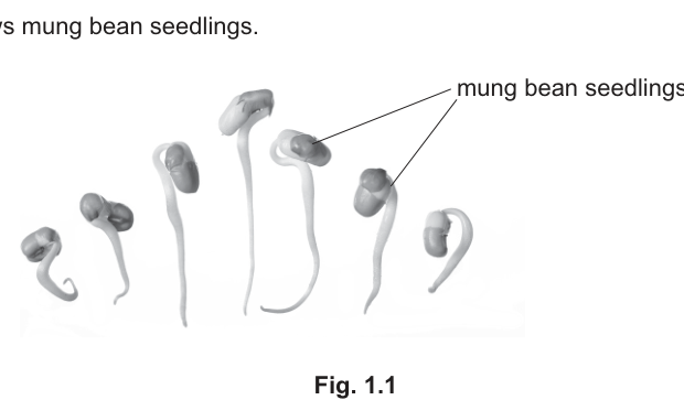
Fig. 1.1

A student found a published method to extract phosphatase from mung bean seedlings.

Use a pestle and mortar to grind mung bean seedlings, with a small volume of distilled water, to make a paste.
Add distilled water to the paste to make a mixture with a total volume of $50\ \text{cm}^3$ .
Filter the mixture and put the filtrate into a clean centrifuge tube.
Centrifuge the filtrate until a solid pellet is formed, as shown in Fig. 1.2.
Pour the liquid extract containing phosphatase into a clean test-tube.

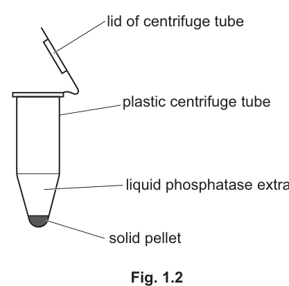
Fig. 1.2

(a)

State two other variables that should be standardised in the published method so that extracts with the same concentration of phosphatase can be produced.

2M Similar

DifficultyEasy

Worked solution

Answer

Any two from:

mass of mung bean seedlings
age / variety / type / cultivar of mung bean seedlings
grinding time (using pestle and mortar)
speed / time in the centrifuge

Final answer

mass of seedlings and age/variety of seedlings (or any two of: mass; age/variety; grinding time; centrifuge speed/time)

Detailed explanation

Background Concept

When an enzyme is extracted from a biological source, the concentration of active enzyme in the final extract depends on more than the protocol itself. The amount of starting material, the physiological state of that material and the vigour with which the cells are disrupted all change the yield. To obtain extracts of reproducible concentration, every one of these factors must be kept constant — they are called standardised (or controlled) variables.

Understanding the Question

The student has a published method for extracting phosphatase from mung bean seedlings and wants the same protocol to give extracts of the same phosphatase concentration each time it is performed. The method already fixes the total volume ( $50\ \text{cm}^{3}$ ), the use of distilled water, filtration, centrifugation to a pellet and decanting the supernatant. We need to suggest two further variables that the user could vary but should not, because they would change the final phosphatase concentration.

Approach

Mentally walk through each step of the published method and ask: "what could I do differently that would change how much phosphatase ends up in the liquid extract?" Then list the most obvious factors and pick two.

Step-by-Step Reasoning

Mass of mung bean seedlings — more tissue means more cells broken open and more enzyme released; a different mass gives a different extract concentration.
Age / variety / cultivar of seedlings — older seedlings contain more cells and more enzyme, and different cultivars can have very different enzyme activities.
Grinding time (pestle and mortar) — longer or harder grinding ruptures more cells and releases more enzyme.
Speed / time in the centrifuge — too low a speed (or too short a time) will not sediment all the cell debris, leaving a more dilute or contaminated extract; too high a speed may sediment some of the enzyme itself.

Any two of these are credited.

Key Takeaways

Standardising variables that affect yield is essential for reproducibility of any extracted-enzyme preparation. The obvious candidates are the amount and type of starting material, the way it is broken up, and the way the extract is clarified.

Common Mistakes

Suggesting variables that are already fixed by the published method (e.g. total volume of $50\ \text{cm}^{3}$ , use of distilled water, filtration).
Suggesting variables that would only affect the assay (e.g. water-bath temperature, pH) rather than the extraction.
Vague answers such as "amount of water" or "the buffer" that are not specified by the protocol.

Things to Be Careful About

The question says "state two other variables". Each must be a specific, named variable — not a paraphrase of the same idea, and not a variable already fixed by the protocol.

Techniques used

identify variables that affect the yield of an extracted enzymeselect variables to standardise to obtain reproducible extracts

(b)

The student read that the optimum pH for phosphatase extracted from mung bean seedlings is less than pH 7.0.

The student decided to investigate phosphatase activity, using the substrate phenolphthalein phosphate (PPP).

In the first four steps of the method, the student:

mixed $5\ \text{cm}^3$ of pH 6.0 buffer solution with $1\ \text{cm}^3$ of a 1.0% solution of PPP in a test-tube
added $1\ \text{cm}^3$ of the phosphatase extract to the test-tube and started a timer
incubated the test-tube for 10 minutes in a water-bath at $30\,^{\circ}\text{C}$
stopped the enzyme reaction after 10 minutes, by adding $5\ \text{cm}^3$ of 10.0% solution of sodium carbonate. Sodium carbonate solution is alkaline.

(i)

The buffered PPP solution and the phosphatase extract were mixed and then placed in the water-bath. The student identified this as a source of error in the method.

Explain why this is a source of error and state how you would modify the method to remove this source of error.

explanation

modification

2M Similar

DifficultyMedium

Worked solution

Answer

Explanation: the temperature of the (mixed) solutions will not have reached $30\,^{\circ}\text{C}$ when the reaction starts, so the rate of reaction will change / not be constant.
Modification: equilibrate the phosphatase (extract) and the PPP (substrate) separately at $30\,^{\circ}\text{C}$ in the water-bath, then mix them and start the timer.

Final answer

Solutions are not at 30 °C when the reaction starts; equilibrate enzyme and substrate separately before mixing.

Detailed explanation

Background Concept

Enzyme reactions are very sensitive to temperature. A meaningful initial-rate measurement is only obtained if the reaction is at a known, constant temperature from the moment it begins. If two reactants are mixed and only then placed in a water-bath, the mixture is below the water-bath temperature at $t = 0$ and warms up during the early part of the reaction; the rate recorded is therefore not the rate at the stated temperature.

Understanding the Question

The student mixes the buffered PPP solution with the phosphatase extract, then puts the test-tube into the $30\,^{\circ}\text{C}$ water-bath. We have to (a) explain why this is a problem and (b) say how to fix it. The question gives one mark for each of these two parts.

Approach

Think about what happens physically when two room-temperature solutions are mixed and put into the bath: the contents are cooler than $30\,^{\circ}\text{C}$ at $t = 0$ and warm up gradually. The clock is already running, so the rate being measured is some kind of average over a range of temperatures, not the rate at $30\,^{\circ}\text{C}$ .

Step-by-Step Reasoning

Explanation: at the moment the timer is started, the mixed solutions are at room temperature, not $30\,^{\circ}\text{C}$ . The reaction therefore begins at a lower temperature and speeds up as the tube warms. The recorded rate is not a true initial rate at $30\,^{\circ}\text{C}$ , and the reaction conditions are not constant during the incubation.
Modification: stand the buffered PPP solution and the phosphatase extract separately in the $30\,^{\circ}\text{C}$ water-bath for a few minutes to equilibrate, then mix them and start the timer. The reaction now begins at $30\,^{\circ}\text{C}$ and the recorded initial rate is the rate at the stated temperature.

Key Takeaways

A genuine "initial rate" requires the reaction to start at the chosen temperature, not warm up to it.
Equilibration of each reactant separately before mixing is the standard fix whenever two solutions are to be combined at a temperature different from room temperature.

Common Mistakes

Saying the reaction would be "too fast" or "too slow" without explaining that the temperature is changing during the reaction.
Suggesting only "put the tube in the water-bath first" — this is what the student is already doing.
Mentioning only one of the two solutions being equilibrated; the mark scheme requires both.

Things to Be Careful About

The mark scheme explicitly requires both solutions to be equilibrated. Credit is not given for "warm up the mixture" because that is the very thing the student is already doing wrong.

Techniques used

identify a source of error in an enzyme assaypropose a modification to control temperature before mixing reactants

(ii)

Suggest how the addition of 10.0% solution of sodium carbonate stops the enzyme reaction.

1M Similar

DifficultyMedium-Easy

Worked solution

Answer

The 10.0% sodium carbonate solution is strongly alkaline; the resulting high pH denatures the phosphatase, so it can no longer catalyse the reaction.

Final answer

The alkaline sodium carbonate denatures the phosphatase.

Detailed explanation

Background Concept

Enzymes are proteins whose tertiary structure is held in the correct 3-D shape by hydrogen bonds, ionic interactions and hydrophobic interactions. Extremes of pH disrupt these interactions so that the active site loses its specific shape. The enzyme is then said to be denatured — it can no longer bind substrate. This is the principle behind many "stop" reagents used in enzyme assays: push the pH far from the enzyme's optimum, and the catalysis halts.

Understanding the Question

The optimum pH of this phosphatase is below 7. The student adds a strongly alkaline 10% sodium carbonate solution to stop the reaction. We have to explain how this stops the catalysis.

Approach

Link the property of sodium carbonate (alkaline / high pH) to its effect on the enzyme (denaturation) to the outcome (no further reaction).

Step-by-Step Reasoning

Sodium carbonate is alkaline; adding it shifts the pH of the reaction mixture well above the optimum (and above pH 7).
At this pH the tertiary structure of the phosphatase is disrupted — the active site loses its specific shape.
The enzyme is denatured and can no longer bind PPP, so the reaction is halted.

Key Takeaways

An extreme of pH is a common and reliable way to terminate an enzyme assay.
"Denature" is the required technical term — saying it "kills", "destroys" or "poisons" the enzyme is too vague and would not score.

Common Mistakes

Saying the sodium carbonate "reacts with" the enzyme or the substrate (it does not — it changes the pH).
Saying the sodium carbonate "neutralises" the enzyme (it does not neutralise, it denatures).
Confusing denaturation (irreversible shape change) with inhibition (reversible binding at the active site).

Things to Be Careful About

Use the word "denature". The mark scheme explicitly rewards this term and rejects weaker language.

Techniques used

explain how alkaline pH inactivates an enzyme

(c)

The phosphatase catalyses the removal of inorganic phosphate from PPP as shown by:

\text{PPP} \xrightarrow{\text{phosphatase}} \text{phenolphthalein} + \text{inorganic phosphate}

The 10.0% solution of sodium carbonate added at the end of the experiment also causes any phenolphthalein to turn pink. The intensity of the pink colour is an indication of the concentration of phenolphthalein.

To estimate the concentration of phenolphthalein produced by the reaction, the student decided to make a proportional dilution using a 2.0% stock solution of phenolphthalein.

The student made $50\ \text{cm}^3$ of each diluted solution.

Describe a method the student could use to make a proportional dilution of the 2.0% stock solution of phenolphthalein to get a range of concentrations.

2M Similar

DifficultyMedium-Easy

Worked solution

Answer

Make five (or more) dilutions, each with a total volume of $50\ \text{cm}^{3}$ , by mixing a stated volume of the 2.0% phenolphthalein stock with a stated volume of distilled water. For example:

Concentration of phenolphthalein (%)	Volume of 2.0% stock (cm³)	Volume of distilled water (cm³)
2.0	50	0
1.5	37.5	12.5
1.0	25	25
0.5	12.5	37.5
0.0	0	50

(For each row, use a pipette / measuring cylinder to measure the volume of stock into a beaker (or flask), add the stated volume of distilled water, and mix thoroughly.)

Final answer

Proportional dilution: stated volumes of 2.0% stock + distilled water, each made up to 50 cm³ (e.g. 37.5 + 12.5 = 50 cm³ of 1.5%; 25 + 25 = 50 cm³ of 1.0%).

Detailed explanation

Background Concept

A proportional (or serial-style) dilution is made by mixing a fixed proportion of a stock solution with a fixed proportion of diluent (here distilled water) so that the final concentration is a known fraction of the stock. Because the total volume is the same for every dilution, the relationship $C_1 V_1 = C_2 V_2$ applies directly: the volume of stock needed is $(C_2 / C_1) \times$ total volume. In this question the stock is 2.0% phenolphthalein and each dilution must be made up to $50\ \text{cm}^{3}$ .

Understanding the Question

The student needs to construct a set of standards of known phenolphthalein concentration so that the concentration of phenolphthalein in an unknown reaction mixture can be read off a calibration curve. The standards must cover the range of interest from the highest expected concentration (close to 2.0%) down to a low (or zero) value, and each must be made to the same final volume so that the colour intensity is comparable.

Approach

Pick a sensible range of concentrations between 2% and 0%, calculate the volume of 2.0% stock required for each using $C_1 V_1 = C_2 V_2$ , and then state the volume of distilled water to make the total up to $50\ \text{cm}^{3}$ .

Step-by-Step Reasoning

For a 1.5% solution: $V_{\text{stock}} = (1.5/2.0) \times 50 = 37.5\ \text{cm}^{3}$ of 2.0% stock, made up to $50\ \text{cm}^{3}$ with $12.5\ \text{cm}^{3}$ of distilled water.
For a 1.0% solution: $V_{\text{stock}} = (1.0/2.0) \times 50 = 25\ \text{cm}^{3}$ of 2.0% stock, plus $25\ \text{cm}^{3}$ of distilled water.
For a 0.5% solution: $V_{\text{stock}} = (0.5/2.0) \times 50 = 12.5\ \text{cm}^{3}$ of 2.0% stock, plus $37.5\ \text{cm}^{3}$ of distilled water.
Repeat for as many intermediate concentrations as desired; the 2.0% and 0.0% end-points are simply the undiluted stock and distilled water respectively.
For each, measure the stock with a pipette (or measuring cylinder), add the stated volume of distilled water, and mix thoroughly.

Key Takeaways

A proportional dilution uses $C_1 V_1 = C_2 V_2$ to find the volume of stock.
Keeping the total volume constant ( $50\ \text{cm}^{3}$ here) means absorbance depends only on concentration, not on path length, so a calibration curve is valid.
At least five different concentrations are needed to draw a reliable calibration curve.

Common Mistakes

Adding the diluent to the stock without making the total up to $50\ \text{cm}^{3}$ (this is the most common error and breaks the proportionality).
Choosing concentrations that do not span the expected range of the reaction mixture (e.g. only 2.0% and 1.0% — too few points and not enough range).
Using a non-linear dilution (e.g. 1.5, 1.2, 0.9, 0.6, 0.3 is acceptable, but the volumes must still be calculated correctly).
Forgetting to include the units (%) when stating the concentrations.

Things to Be Careful About

The mark scheme requires (1) five stated concentrations between 2% and 0% with units, and (2) the correct method of dilution shown for two of them. A clear table satisfies both requirements at once.

Techniques used

calculate dilution volumes using C1V1 = C2V2prepare a proportional dilution series from a stock solution

(d)

Describe how the student could use the dilutions from (c) and a colorimeter to estimate the concentration of phenolphthalein in a reaction mixture.

2M Similar

DifficultyMedium-Easy

Worked solution

Answer

Zero the colorimeter using a blank (e.g. distilled water, or sodium-carbonate/buffer without phenolphthalein).
Measure the absorbance of each of the standard dilutions from (c) and the absorbance of the reaction mixture, using a suitable filter (green for pink colour).
Plot a calibration curve of absorbance (y-axis) against phenolphthalein concentration (x-axis) for the standard dilutions, and read off the concentration of phenolphthalein in the reaction mixture from the curve.

Final answer

Measure absorbance of standards and reaction mixture; read concentration of the reaction mixture from a calibration curve of absorbance vs phenolphthalein concentration.

Detailed explanation

Background Concept

A colorimeter measures how much light of a chosen wavelength is transmitted through a sample; it displays this as absorbance, which is proportional to the concentration of the absorbing species (Beer–Lambert law). If a set of standards of known concentration is measured in the same instrument under the same conditions, a graph of absorbance against concentration (the calibration curve) can be used to look up the concentration of an unknown sample from its absorbance.

Understanding the Question

The student has a series of phenolphthalein standards of known concentration (from part (c)) and a reaction mixture whose phenolphthalein concentration is unknown. We have to describe how a colorimeter and the standards can be combined to estimate that unknown concentration.

Approach

The classic three steps: zero the instrument, measure the standards and the unknown in the same way, then read the unknown from a calibration curve.

Step-by-Step Reasoning

Set the colorimeter to a wavelength (or filter) that the pink phenolphthalein absorbs strongly — a green filter is the typical choice for a pink solution.
Zero the colorimeter with a blank cuvette containing everything except phenolphthalein (e.g. distilled water, or a mixture of buffer and sodium carbonate). This corrects for any background absorbance from the solvent, the cuvette and the reagents.
Measure the absorbance of each standard dilution from (c); these are the points of the calibration curve.
Measure the absorbance of the reaction mixture in the same cuvette using the same filter.
Plot absorbance (y) against phenolphthalein concentration / % (x) for the standards, draw a smooth best-fit line, and read the concentration of the reaction mixture off the line at its measured absorbance.

Key Takeaways

A blank is essential — without it, the readings include background absorbance and the calibration is invalid.
A calibration curve must be constructed from at least five standards covering the expected range.
The filter colour should be the complementary colour of the solution (green for pink).

Common Mistakes

Forgetting to use a blank (so absorbance readings include the cuvette and the solvent).
Plotting concentration on the y-axis and absorbance on the x-axis (the convention is the other way round, and the unknown is read off the x-axis).
Measuring the standards and the unknown with different filters or different path lengths (cuvettes must be matched).
Drawing a straight line through the origin and the highest standard only, instead of fitting all the points.

Things to Be Careful About

The mark scheme requires both measuring the absorbance of the dilutions and the reaction mixture, and using the calibration curve to determine the concentration — two distinct points.

Techniques used

use a colorimeter to measure absorbanceconstruct and use a calibration curve to determine an unknown concentration

(e)

The student decided to determine the optimum pH for phosphatase extract from the mung bean seedlings.

Describe a method the student could use to determine the optimum pH for phosphatase.

Your method should be set out in a logical order and be detailed enough to allow another person to follow it.

Details of how to extract phosphatase from the mung bean seedlings and how to make the dilutions of phenolphthalein solutions should not be included.

6M Similar

DifficultyMedium-Hard

Worked solution

Answer

Prepare buffer solutions. Prepare five buffer solutions of known, different pH values covering the range of interest up to pH 7 (e.g. pH 3, 4, 5, 6 and 7).
Equilibrate. Place each buffered PPP solution and the phosphatase extract separately in a $30\,^{\circ}\text{C}$ water-bath for a few minutes to equilibrate to the incubation temperature.
Mix and incubate. Add a fixed volume (e.g. $1\ \text{cm}^{3}$ ) of the phosphatase extract to a fixed volume (e.g. $5\ \text{cm}^{3}$ ) of PPP + buffer at the chosen pH, mix, and start a timer. Incubate at $30\,^{\circ}\text{C}$ for a fixed time (e.g. 10 min).
Stop the reaction. Add $5\ \text{cm}^{3}$ of 10.0% sodium carbonate solution to halt the reaction.
Calibrate the colorimeter. Zero the colorimeter (with a filter suitable for the pink colour) using a blank cuvette containing water (or buffer + sodium carbonate without PPP).
Measure absorbance. Measure the absorbance of each reaction mixture and record it against the corresponding pH.
Identify the apparent optimum. Plot absorbance (y) against pH (x) and identify the pH that gives the highest absorbance as the apparent optimum.
Refine the range. Repeat the experiment using smaller pH intervals (e.g. 0.2 pH units) around the apparent optimum to pinpoint it more accurately.
Replicate and average. Repeat the whole experiment at least twice at each pH and calculate a mean absorbance for each pH.
Safety. Sodium carbonate / strong buffers / PPP are irritant; wear gloves and eye protection.

Final answer

See working — a full plan covering pH buffers, equilibration, mixing, colorimeter calibration, fixed-time incubation, identification of the optimum, refinement around the optimum, replication and a stated safety precaution.

Detailed explanation

Background Concept

Every enzyme has an optimum pH at which its active site has the correct shape and charge, and at which the rate of the reaction it catalyses is therefore highest. The pH optimum is found by measuring the activity of the enzyme at a range of pH values while keeping all other variables (temperature, substrate concentration, enzyme concentration, incubation time) constant. Activity is read out as the concentration of product (here, phenolphthalein) formed in a fixed time, and is most conveniently measured by absorbance in a colorimeter.

Understanding the Question

The student wants a method that will determine the pH at which the phosphatase extract is most active. The method has to be detailed enough for another person to follow, but extraction and dilution procedures are excluded (they have been described in earlier parts). The plan must therefore start from the ready-made extract and the ready-made phenolphthalein standards.

Approach

A plan to determine an optimum needs:

a range of values for the independent variable (pH);
control of every other variable (temperature, volumes, time);
a quantitative measure of activity (absorbance via colorimeter);
replication and a mean;
a way to refine the answer near the apparent optimum;
a safety point.

Step-by-Step Reasoning

Buffer range: at least five pH values up to pH 7 are needed so the optimum can be located; the question states the optimum is below pH 7.
Equilibration: if the buffered substrate and the enzyme are mixed at room temperature and only then placed in the water-bath, the initial rate is not at the stated temperature (the same error discussed in (b)(i)). Equilibrating both separately fixes this.
Fixed volumes and time: the volume of buffer + PPP and the volume of enzyme extract must be the same at every pH, and the incubation time must be the same, so that any difference in absorbance is due to pH alone.
Stopping the reaction: sodium carbonate is the stop reagent (alkaline, denatures the enzyme, see (b)(ii)).
Colorimeter zeroing: a blank removes background absorbance from buffer + sodium carbonate; without a blank the readings are not comparable.
Identifying the optimum: plot absorbance against pH; the highest absorbance is the apparent optimum.
Refining: if the apparent optimum falls between, say, pH 5 and 6, repeat the experiment at pH 5.0, 5.2, 5.4, 5.6, 5.8, 6.0 to find the true maximum.
Replication: repeating the experiment at each pH and calculating a mean reduces the effect of random error and lets outliers be identified.
Safety: sodium carbonate is irritant to skin and eyes; PPP and the extract are also irritant / potential allergens. Gloves and eye protection are the standard precaution.

Key Takeaways

An optimum is found by holding every variable constant except one (the independent variable) and measuring the dependent variable across a range.
Equilibration, calibration and replication are the three reliability points that almost every enzyme-assay plan must include.
A plan must be detailed enough to be followed by another person — vague steps ("test different pHs") do not score.

Common Mistakes

Forgetting to equilibrate the reactants before mixing (the same error as in (b)(i)).
Using the same colorimeter reading for all pHs without re-zeroing with a fresh blank (the blank must be matched to the new buffer at each pH, or a single buffer blank used — but the calibration step must be mentioned).
Not specifying a fixed incubation time, so the reaction runs to different extents at different pHs.
Failing to refine the range around the apparent optimum (the answer cannot be given to better than the step size of the original pH series).
Forgetting replication or a mean.
Omitting a named hazard and a specific precaution.

Things to Be Careful About

The mark scheme accepts any six of nine credited points; the list above covers all nine, so the plan is robust to any small omission by the candidate. The phrasing must be in a logical order (preparation → equilibration → mixing → measurement → analysis) for full credit.

Techniques used

plan an investigation to determine the optimum pH of an enzymecontrol variables and equilibrate reactantsuse a colorimeter with a blank to compare treatmentsrefine the range of pH around the apparent optimum and calculate means

(f)

The student investigated the effect of a competitive inhibitor on the activity of a phosphatase.

Fig. 1.3 shows a graph of the initial rates of enzyme reaction against PPP concentration for the enzyme with no inhibitor and the enzyme with inhibitor.

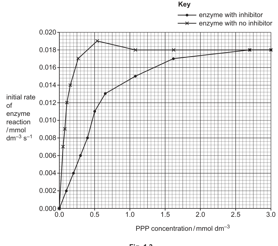
Fig. 1.3

(i)

One of the data plots in Fig. 1.3 is anomalous.

Circle the anomalous data plot in Fig. 1.3 and explain why you think it is anomalous.

2M Similar

DifficultyMedium

Worked solution

Answer

Circle the data point at PPP concentration $= 0.5\ \text{mmol dm}^{-3}$ on the "enzyme with no inhibitor" curve (rate $\approx 0.019\ \text{mmol dm}^{-3}\ \text{s}^{-1}$ ).

This point is anomalous because it is higher than $V_{\text{max}}$ (the plateau at $\approx 0.018\ \text{mmol dm}^{-3}\ \text{s}^{-1}$ ). The rate of an enzyme-catalysed reaction cannot exceed $V_{\text{max}}$ , so a value above the plateau must be a measurement error.

Final answer

The point at PPP = 0.5 mmol dm⁻³ (rate ≈ 0.019) on the no-inhibitor curve is anomalous because it is above the Vmax plateau (~0.018).

Detailed explanation

Background Concept

In a Michaelis–Menten plot of initial rate against substrate concentration, the curve rises steeply at low [S] and levels off at high [S] to a plateau called $V_{\text{max}}$ . $V_{\text{max}}$ is the rate at which the enzyme is saturated with substrate — every active site is occupied, so the rate is limited by the amount of enzyme and cannot be exceeded by adding more substrate. Any data point that lies above the plateau is therefore a measurement error, not a real feature of the reaction.

Understanding the Question

Fig. 1.3 shows two Michaelis–Menten curves, one without inhibitor and one with a competitive inhibitor. The candidate must identify the single data point that does not fit its curve and explain why it is anomalous. The printed figure itself is to be annotated.

Approach

Look at each curve in turn and ask whether the trend makes sense. The "no inhibitor" curve plateaus at $V_{\text{max}} \approx 0.018\ \text{mmol dm}^{-3}\ \text{s}^{-1}$ , and the "with inhibitor" curve eventually approaches the same plateau. Any data point that lies above the plateau of its curve is automatically anomalous, because rates cannot exceed $V_{\text{max}}$ .

Step-by-Step Reasoning

The "no inhibitor" curve should rise and plateau at about $0.018\ \text{mmol dm}^{-3}\ \text{s}^{-1}$ .
The 6th data point on this curve, at PPP concentration $0.5\ \text{mmol dm}^{-3}$ , has a rate of about $0.019\ \text{mmol dm}^{-3}\ \text{s}^{-1}$ — clearly above the plateau.
This is biologically impossible (rate cannot exceed $V_{\text{max}}$ ) and so the point is anomalous, almost certainly a measurement or plotting error.
No other data point lies outside the expected pattern of its curve, so this is the only anomaly.

Key Takeaways

A data point above the $V_{\text{max}}$ plateau is by definition anomalous.
Anomalies are usually identified by visual inspection of a scatter of points against a smooth curve, then justified by an argument about what the data should look like.
The convention when annotating a printed figure is to circle the point, not to redraw the figure.

Common Mistakes

Circling a point simply because it is "off the line" without giving a biological reason why it is impossible.
Circling a point on the "with inhibitor" curve that is in fact on the smooth trend of that curve.
Citing "human error" or "a mistake" without explaining the impossibility (rate > $V_{\text{max}}$ ).

Things to Be Careful About

The mark scheme requires both: the correct point circled, and a reason that mentions $V_{\text{max}}$ / 0.018 / the plateau.

Techniques used

identify an anomalous data point on a graphinterpret a Michaelis–Menten curve and the meaning of Vmax

(ii)

Use Fig. 1.3 to determine the Michaelis–Menten constant ( $K_m$ ) for the enzyme with no inhibitor and for the enzyme with inhibitor.

Include the correct units in your answers.

$K_m$ for the enzyme with no inhibitor = ______
$K_m$ for the enzyme with inhibitor = ______

1M Similar

DifficultyMedium

Worked solution

Answer

$V_{\text{max}}$ for both curves $\approx 0.018\ \text{mmol dm}^{-3}\ \text{s}^{-1}$ , so $\frac{1}{2} V_{\text{max}} \approx 0.009\ \text{mmol dm}^{-3}\ \text{s}^{-1}$ .

Reading the substrate concentration at this rate off each curve:

$K_{\text{m}}$ for the enzyme with no inhibitor $\approx 0.075\ \text{mmol dm}^{-3}$
$K_{\text{m}}$ for the enzyme with inhibitor $\approx 0.425\ \text{mmol dm}^{-3}$

Final answer

Km (no inhibitor) ≈ 0.075 mmol dm⁻³; Km (with inhibitor) ≈ 0.425 mmol dm⁻³

Detailed explanation

Background Concept

The Michaelis–Menten constant $K_{\text{m}}$ is defined as the substrate concentration at which the initial rate of an enzyme-catalysed reaction is half of $V_{\text{max}}$ . On a Michaelis–Menten plot it is read off by drawing a horizontal line at $\frac{1}{2} V_{\text{max}}$ and noting where it meets the curve; the corresponding x-value is $K_{\text{m}}$ . $K_{\text{m}}$ is a measure of the apparent affinity of the enzyme for its substrate: a high $K_{\text{m}}$ means the enzyme needs a lot of substrate to reach half its maximum rate (low apparent affinity), and a low $K_{\text{m}}$ means the opposite.

Understanding the Question

The two curves in Fig. 1.3 both plateau at the same $V_{\text{max}}$ , but they rise at very different rates. The candidate has to read $K_{\text{m}}$ off each curve and quote it with the correct unit.

Approach

Find $V_{\text{max}}$ (the plateau of the curves), halve it, draw a horizontal line at that height, and read off the substrate concentration where the line meets each curve.

Step-by-Step Reasoning

The plateau of both curves is at about $0.018\ \text{mmol dm}^{-3}\ \text{s}^{-1}$ , so $V_{\text{max}} \approx 0.018\ \text{mmol dm}^{-3}\ \text{s}^{-1}$ .
Half of this is $\frac{1}{2} V_{\text{max}} \approx 0.009\ \text{mmol dm}^{-3}\ \text{s}^{-1}$ .
On the "no inhibitor" curve, the rate first reaches $0.009$ at a substrate concentration of about $0.075\ \text{mmol dm}^{-3}$ — so $K_{\text{m,no\ inhibitor}} \approx 0.075\ \text{mmol dm}^{-3}$ .
On the "with inhibitor" curve, the rate does not reach $0.009$ until the substrate concentration is about $0.43\ \text{mmol dm}^{-3}$ (between 0.4 and 0.5, closer to 0.4) — so $K_{\text{m,with\ inhibitor}} \approx 0.425\ \text{mmol dm}^{-3}$ (or $0.43\ \text{mmol dm}^{-3}$ ).
The unit is the unit of the x-axis: $\text{mmol dm}^{-3}$ .

Key Takeaways

$K_{\text{m}}$ is the substrate concentration at $\frac{1}{2} V_{\text{max}}$ , read off a Michaelis–Menten curve.
A competitive inhibitor increases $K_{\text{m}}$ (the enzyme appears to have a lower affinity for its substrate) but does not change $V_{\text{max}}$ (which the curves confirm).
Always quote $K_{\text{m}}$ with the unit of the x-axis.

Common Mistakes

Confusing $K_{\text{m}}$ with the substrate concentration at $V_{\text{max}}$ (which would be the x-value of the plateau — that has no special meaning).
Reading $K_{\text{m}}$ off at the wrong rate (e.g. at $V_{\text{max}}$ itself, or at one third $V_{\text{max}}$ ).
Forgetting the unit, or quoting it as the y-axis unit ( $\text{mmol dm}^{-3}\ \text{s}^{-1}$ ).
Reversing the two values (assigning the larger $K_{\text{m}}$ to the no-inhibitor curve).

Things to Be Careful About

The mark scheme accepts both $0.43$ and $0.425$ for the inhibited $K_{\text{m}}$ , reflecting the limited precision of a graph read. Always state the unit ( $\text{mmol dm}^{-3}$ ).

Techniques used

read Km from a Michaelis–Menten graphinterpret the meaning of the Michaelis–Menten constant

(iii)

Calculate the percentage increase in the $K_m$ that occurs in the presence of the inhibitor.

Show your working.

percentage increase = ______ %

2M Similar

DifficultyMedium-Easy

Worked solution

Working

\text{percentage increase} = \frac{K_{\text{m,with\ inhibitor}} - K_{\text{m,no\ inhibitor}}}{K_{\text{m,no\ inhibitor}}} \times 100

= \frac{0.425 - 0.075}{0.075} \times 100

= \frac{0.350}{0.075} \times 100 = 466.67\%

Answer

percentage increase $\approx 467\%$

Final answer

≈ 467% (accept 467–473% depending on whether 0.425 or 0.43 is used for Km with inhibitor)

Detailed explanation

Background Concept

Percentage change between two values is calculated as $\frac{\text{new} - \text{original}}{\text{original}} \times 100$ . In this case the "new" value is the $K_{\text{m}}$ measured in the presence of the inhibitor, and the "original" is the $K_{\text{m}}$ without inhibitor. The result quantifies how much the inhibitor has decreased the apparent affinity of the enzyme for its substrate.

Understanding the Question

The candidate has the two $K_{\text{m}}$ values from (f)(ii) and is asked to express the difference as a percentage of the original (no-inhibitor) value.

Approach

Substitute into the percentage change formula and evaluate.

Step-by-Step Reasoning

Difference: $0.425 - 0.075 = 0.350\ \text{mmol dm}^{-3}$ .
Divide by the original value: $0.350 / 0.075 = 4.6667$ .
Multiply by 100: $4.6667 \times 100 = 466.67\%$ .
Rounded to three significant figures: $467\%$ .

(If $0.43$ is used for the inhibited $K_{\text{m}}$ instead, the answer is $\frac{0.43 - 0.075}{0.075} \times 100 = 473\%$ , which the mark scheme also accepts.)

Key Takeaways

Percentage change is always expressed relative to the original (control) value, not the new one.
The answer should be quoted to the same number of significant figures as the input data (three here).

Common Mistakes

Dividing by the wrong value (e.g. by the inhibited $K_{\text{m}}$ instead of the no-inhibitor $K_{\text{m}}$ ).
Quoting a fraction (4.67) instead of a percentage (467%).
Rounding too early and giving an inaccurate answer (e.g. 460%).
Using the wrong operation (e.g. ratio rather than percentage change).

Things to Be Careful About

Show the working explicitly — the mark scheme credits the working separately from the final numerical answer, so an answer with no working can only earn the second mark if it is exactly right.

Techniques used

calculate percentage increase between two values

Q2Medium-HardPlanningAnalysis, Conclusions and Evaluation

Sponges are immobile, aquatic animals that live on rocks and sediment at the bottom of salt water environments.

Fig. 2.1 shows an example of a sponge, growing on the seabed, in a marine habitat.

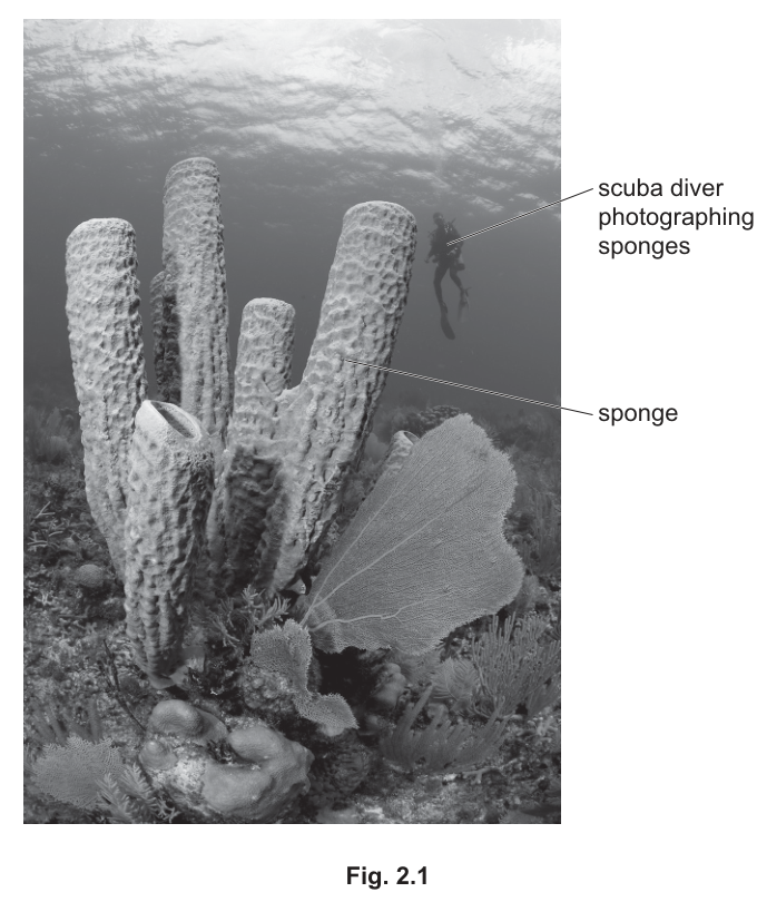
Fig. 2.1

There are many different species of sponge. Most species of sponge are sensitive to environmental stress. Human activity causes some environmental stress.

(a)

Scientists sampled the marine habitats along a length of coastline in Algeciras Bay in southern Spain to study the species diversity of sponges.

The scientists selected 12 sampling stations, A to L, as shown in Fig. 2.2. The scientists noted the land use or human activity along the coast next to each sampling station.

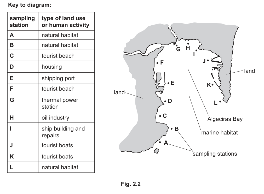
Fig. 2.2

The sampling stations were chosen to compare the effects of land use or human activity on the species diversity of sponges in the bay.

At each marine sampling station, the scientists:

placed permanent line transects, $50\ \text{m}$ in length, on the seabed
photographed all sponges sighted at a distance of $1\ \text{m}$ either side of the transect
sampled each transect for the same length of time
sampled each transect four times a year.

The scientists standardised some variables.

State two other variables that the scientists should standardise in this investigation.

2M Similar

DifficultyMedium-Easy

Worked solution

Answer

(The same) time of year / season / month ;
(The same) depth of, water / sea / sponge / seabed / water pressure ;

(Other credit: same orientation of transect)

Final answer

(Same) time of year/season; 2. (Same) depth of water.

Detailed explanation

Background Concept

In an investigation comparing species diversity between sites, variables other than the independent variable (here, type of land use / human activity) must be kept constant. If a confounding variable differs between sites, any difference in the dependent variable (sponge species diversity) could be due to the confounder rather than the named treatment. Standardising these variables improves the validity of the comparison.

Sponges are sessile (immobile) filter-feeders. Their distribution is strongly affected by abiotic factors such as:

Water depth and pressure — different species are adapted to different depth zones; light penetration, pressure and temperature all change with depth.
Season / time of year — temperature, plankton availability (their food) and breeding cycles vary seasonally, which can change the species present or visible.
Substrate type and orientation — sponges colonise hard surfaces; the orientation of the substrate affects light and current exposure, which influences which species can settle.

Understanding the Question

The scientists have already standardised several things: transect length (50 m), distance either side (1 m), sampling time, and sampling frequency (four times a year). The question asks for two further variables that should be standardised so that the comparison of sponge species diversity between stations is fair.

The command word is state — a brief, factual answer is enough; no explanation is required.

Approach

Think about environmental or methodological factors that could vary between the 12 stations and that influence what sponges are present (or detectable). Pick two from the list the mark scheme accepts.

Step-by-Step Reasoning

Time of year / season / month — sponge species may appear, reproduce or be more visible at certain times of year. Sampling all stations in the same season removes this source of variation.
Depth of water / sea / sponge / seabed / water pressure — different sponge species live at different depths. If station A is at 5 m and station G is at 25 m, depth differences could drive the diversity difference rather than the land use. Standardising depth controls for this.
(Alternative credit) Orientation of transect — e.g. all transects running parallel to the shore, since aspect affects light and current.

Key Takeaways

In comparative ecological studies, the only difference between sites should be the independent variable.
Depth and season are two of the most important confounders in marine surveys.
"Standardise" means actively controlling a variable, not just measuring it.

Common Mistakes

Naming variables that have already been standardised in the question (transect length, time spent sampling, frequency, distance) — these earn no credit because they are given.
Vague answers such as "the same conditions" or "the same environment" — these are not specific enough to score.
"Same number of divers" or "same equipment" — these are possible controls but the mark scheme only credits the listed alternatives.

Things to Be Careful About

The question says "two other variables", so credit is only given for variables that have not already been mentioned in the procedure.
Use the precise wording on the mark scheme; for example, "depth of water" or "depth of seabed" both score, but a vague "water conditions" does not.

Techniques used

identify standardised variables in an ecological investigationsuggest controls for a transect-based sampling studyapply knowledge of factors affecting marine organisms

(b)

The scientists compared the species diversity of sponges between different sampling stations using an index of diversity known as beta diversity.

The higher the beta diversity index, the higher the species diversity at a sampling station.

Fig. 2.3 shows a graph of the beta diversity index for each sampling station.

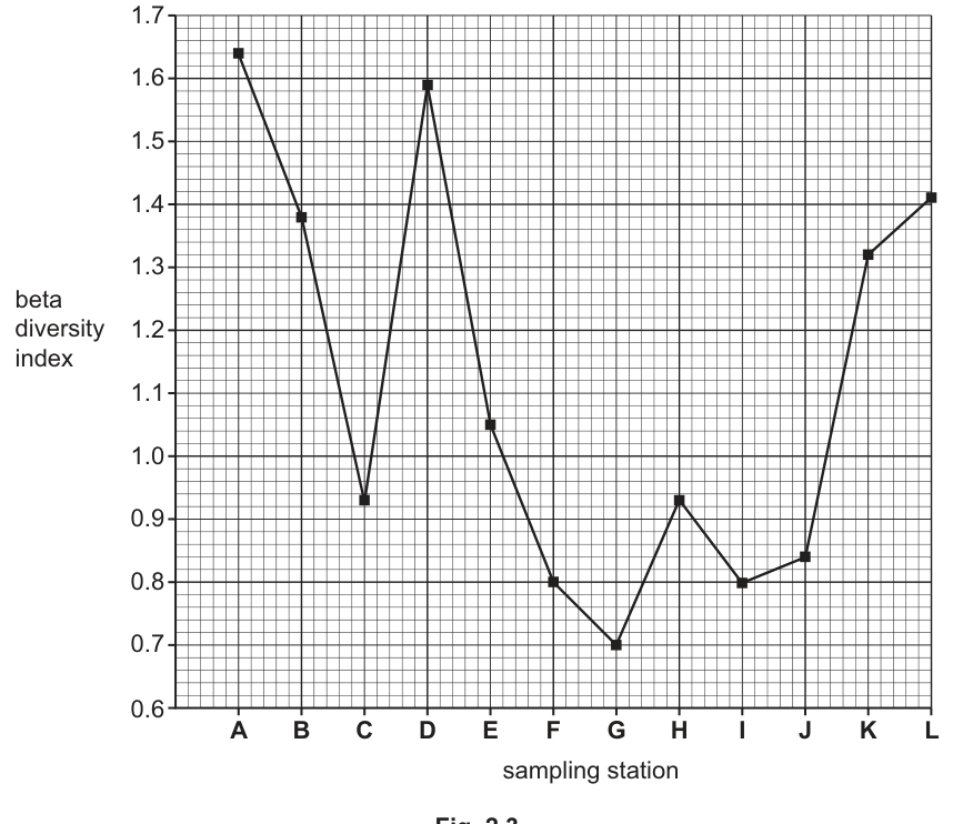
Fig. 2.3

A simplified formula for beta diversity is shown:

\text{beta diversity} = \frac{n}{\bar{x} - 1}

Key to symbols:
$n$ = the number of sponge species recorded at a sampling station
$\bar{x}$ = the mean number of sponge species across all sampling stations

At sampling station A, 37 sponge species were recorded ( $n = 37$ ).

Use Fig. 2.3 and the formula for beta diversity to calculate the mean number of sponge species across all sampling stations ( $\bar{x}$ ).

Show your working. Write your answer to the nearest whole number.

mean number of sponge species across all sampling stations ( $\bar{x}$ ) = ______

2M Similar

DifficultyMedium

Worked solution

Working

From Fig. 2.3, the beta diversity index at station A = 1.64

At A, $n = 37$ species.

\text{beta diversity} = \frac{n}{\bar{x} - 1}

1.64 = \frac{37}{\bar{x} - 1}

\bar{x} - 1 = \frac{37}{1.64} = 22.56

\bar{x} = 22.56 + 1 = 23.56

Rounded to the nearest whole number:

Answer

$\bar{x} = 24$ (allow 23)

Final answer

Detailed explanation

Background Concept

Beta diversity is a measure of species diversity at a site. The simplified formula used here is

\text{beta diversity} = \frac{n}{\bar{x} - 1}

where $n$ is the number of species at one station and $\bar{x}$ is the mean number of species across all stations sampled. Rearranging the formula lets you calculate $\bar{x}$ from a single data point if you also know the index at that point.

Understanding the Question

You are told:

$n = 37$ at station A.
The beta diversity index at A is on the graph (Fig. 2.3).
The formula links the two with the unknown $\bar{x}$ .

The task is a calculation with working shown and the answer given to the nearest whole number.

Approach

Read the beta diversity value at A off the graph.
Substitute into the formula.
Rearrange to make $\bar{x}$ the subject.
Round to the nearest whole number.

Step-by-Step Reasoning

Step 1 — Read the graph. Station A is the leftmost point. Its beta diversity index is approximately 1.64 (accept 1.6 if the candidate's reading is slightly different).

Step 2 — Substitute.

1.64 = \frac{37}{\bar{x} - 1}

Step 3 — Rearrange. Multiply both sides by $(\bar{x} - 1)$ and divide by 1.64:

\bar{x} - 1 = \frac{37}{1.64} = 22.56

Then add 1:

\bar{x} = 23.56

Step 4 — Round to the nearest whole number. $23.56$ rounds to 24. (The mark scheme accepts 23 or 24 because small differences in reading the graph give $\bar{x}$ values between 22.6 and 24.0.)

Key Takeaways

The mark scheme awards one mark for the correct final answer (23 or 24) and one mark for the working — both must be visible.
Always show the substitution into the formula so the examiner can award "correct working" even if the numerical answer is slightly off.
Reading graphs: use the gridlines to read the value as accurately as you can. The y-axis here is in 0.02 increments between major lines of 0.1.

Common Mistakes

Forgetting to add 1 at the end (giving an answer around 22.6).
Writing only the final answer with no working.
Misreading the value at A (e.g. 1.6 or 1.7), which is acceptable as long as the working is consistent.

Things to Be Careful About

The "nearest whole number" instruction matters: 23.56 → 24, not 23.
The mark scheme allows a small tolerance because the graph is read by eye. Both 23 and 24 are accepted.
The formula uses $\bar{x} - 1$ , not $\bar{x}$ alone; missing the $-1$ loses both marks.

Techniques used

read a value from a line graphrearrange a formula to make a variable the subjectsubstitute numerical values into an equationround a calculated value to a whole number

(c)

(i)

A student concluded that the species diversity of sponges was higher in the sampling stations where there was less human activity.

Using the information in Fig. 2.2 and in Fig. 2.3, evaluate this conclusion.

Use the values in Fig. 2.3 to support your answer.

3M Similar

DifficultyMedium-Hard

Worked solution

Answer

Evidence supporting the conclusion (human activity = lower diversity):

Station A (natural habitat) has the highest beta diversity index, 1.64 ;
Station G (thermal power station) has the lowest index, 0.70 ;
The three natural-habitat stations A, B, L all have higher indices (1.64, 1.38, 1.41) than the stations inside the bay with heavy industry / shipping.

Evidence not supporting the conclusion (so the conclusion is only partially valid):

D (housing) has a similar / higher beta diversity index (1.59) than the natural-habitat station A (1.64) and higher than B (1.38) and L (1.41) — so housing does not reduce diversity here ;
J and K have the same human activity (tourist boats) but very different indices (0.84 vs 1.32) — therefore the same activity does not always produce the same effect ;
The index only counts the number of species, not the number of individuals; a more rigorous measure such as Simpson's index of diversity would also account for relative abundance.

Evaluation: The conclusion is partly supported. Natural-habitat stations generally have higher diversity and the lowest value is at a heavily industrial site, but the effect is not consistent across all stations of the same land-use type.

Final answer

Conclusion is partly supported: natural-habitat stations A, B, L generally have higher beta diversity indices (1.64, 1.38, 1.41) and station G (thermal power station) has the lowest (0.70); but D (housing, 1.59) is similar to or higher than natural habitats, and J and K (same activity — tourist boats) differ (0.84 vs 1.32). The index also only counts species number, not abundance.

Detailed explanation

Background Concept

Evaluating a conclusion means weighing up the evidence for and against a claim, rather than just describing whether the data agree with it. A good evaluation:

States the conclusion being tested.
Gives data that support it.
Gives data that do not support it (or shows the data are inconclusive).
Identifies any limitations of the method that affect how far the conclusion can be trusted.

The beta diversity index used here is calculated as $n / (\bar{x} - 1)$ . It is a measure of how species-rich a site is relative to the average, but the simplified version used here only takes account of the number of species, not how many individuals of each species are present.

Simpson's index of diversity $D = 1 - \sum (n/N)^2$ takes both species richness and evenness (relative abundance) into account and is the more rigorous diversity measure used in A-level Biology.

Understanding the Question

The student's claim: "species diversity of sponges was higher in the sampling stations where there was less human activity." You must evaluate this using the land-use table (Fig. 2.2) and the graph (Fig. 2.3), giving values from the graph to support your answer.

The mark scheme rewards:

One mark for any correct use of the data to qualify a statement.
One mark for evidence that supports the conclusion.
One mark for evidence that does not support the conclusion, or a limitation of the index.

Approach

Look at the natural-habitat stations (A, B, L) and the most industrial stations (E, G, H, I) and compare.
Find one or two clear pieces of evidence that fit the student's claim.
Find one or two clear pieces of evidence that do not fit — these are the key to "evaluate".
Mention the limitation of the index.

Step-by-Step Reasoning

Supporting the conclusion:

Station A (natural habitat) has the highest index, 1.64 — the most undisturbed site has the most diverse sponges.
Station G (thermal power station) has the lowest index, 0.70 — the most industrial site has the least diverse sponges.
The three natural-habitat stations (A, B, L) all have indices ≥ 1.38, generally above the industrial/shipping stations (E, F, G, H, I, J, K all below 1.05 except H at 0.93).

Not supporting the conclusion:

Station D (housing) has a beta diversity index of 1.59, which is essentially the same as the natural-habitat station A (1.64) and higher than B (1.38) and L (1.41). So housing activity does not seem to reduce diversity here.
Stations J and K have the same human activity (tourist boats) but very different indices — J ≈ 0.84 and K ≈ 1.32. The same activity does not produce the same result, so the simple claim "less human activity = higher diversity" is too sweeping.

Limitation of the method:

The index used here only counts the number of species, not the number of individuals of each species. A site could have 20 species but be dominated by 1 species with the other 19 represented by single individuals — it would score as diverse even though the community is heavily dominated. Simpson's index of diversity would be a more informative measure.

Synthesis: The conclusion is partly supported but is an over-simplification. The data are consistent with industrial activity reducing diversity (G is lowest), but housing does not follow the same pattern, and stations with the same land use (J, K) give very different results, so other factors (location within the bay, water currents, etc.) must also be at work.

Key Takeaways

Evaluation = evidence for + evidence against + (if possible) methodological limitation.
Always quote graph values (with units of the index, here dimensionless) to support an argument.
A single anomaly can refute a sweeping claim — point to it explicitly.
Different indices measure different things; knowing the limitation of the index used is part of a complete evaluation.

Common Mistakes

Only describing data that support the conclusion (this is description, not evaluation).
Saying "the conclusion is wrong" without giving a specific counter-example.
Failing to quote numerical values — the mark scheme explicitly requires values from Fig. 2.3.
Citing limitations not on the mark scheme, e.g. "sample size is too small", which is not creditable here.

Things to Be Careful About

The mark scheme allows either a counter-example from the data (D vs A; J vs K) OR a comment about the index. You only need one for the third mark, but giving both is safe.
"Natural habitat" stations are A, B, L — not just A. The student claim is about all less-disturbed sites, so a comparison of all three is stronger evidence than picking one.

Techniques used

evaluate a conclusion against the datause graph values to support an argumentidentify evidence that both supports and contradicts a claimrecognise a limitation of the index used

(ii)

Use the information in Fig. 2.2 and in Fig. 2.3 to state two other conclusions about the species diversity of sponges in Algeciras Bay.

Use the values in Fig. 2.3 to support your answer.

3M Similar

DifficultyMedium

Worked solution

Answer

(Each conclusion must be supported by values from Fig. 2.3.)

Conclusion 1 — The species diversity of sponges is lower inside Algeciras Bay than at stations on the open coast.

Stations on the open coast / at the mouth of the bay (A, B, L) have higher beta diversity indices (1.64, 1.38, 1.41).
Stations within the bay (E, F, G, H, I, J) have lower indices (0.70–1.05).

Conclusion 2 — Industrial activity is associated with lower species diversity.

Industrial stations E, G, H, I (shipping port, thermal power station, oil industry, ship building) all have low indices (0.70–1.05), lower than the natural-habitat stations A, B, L (≥ 1.38).

Conclusion 3 — Tourism has a variable effect on diversity.

Tourist-beach stations C and F have low indices (0.93, 0.80) but tourist-boat stations J (0.84) and K (1.32) differ markedly — so tourism does not consistently lower diversity.

Conclusion 4 — Housing has less effect on diversity than other human activities.

Station D (housing) has a high index (1.59), similar to natural habitats and higher than most other human-activity stations.

Final answer

Diversity is higher at open-coast stations A, B, L (indices 1.64, 1.38, 1.41) than inside the bay (E–J mostly 0.70–1.05). 2. Industrial stations (E, G, H, I) have low indices (0.70–1.05), lower than the natural-habitat stations. (Other credit: tourism's effect is variable; housing D has an index similar to natural habitats.)

Detailed explanation

Background Concept

A conclusion is a statement that is directly supported by the data. It should:

Be specific (about a particular feature of the data, not vague).
Be supported by quoted values.
Not overreach beyond what the data show.

The mark scheme specifically requires the conclusion to be about species diversity of sponges — not about the index itself, and not about "biodiversity". The simplified beta diversity index used here reflects species richness (number of species), so the conclusion is most safely phrased in terms of the number of species / species diversity rather than abundance.

Understanding the Question

Using Fig. 2.2 (the map + key) and Fig. 2.3 (the graph), state two other conclusions about sponge species diversity. "Other" means not the conclusion that the student already drew (that diversity is higher where there is less human activity). Each conclusion must be backed up by values from the graph.

The mark scheme awards:

1 mark for quoting correct index data to support a conclusion.
Up to 2 further marks for any two of the listed alternative conclusions.

Approach

Group the 12 stations by something other than the simple "human vs natural" split the student used.
Look for a pattern within each group.
Quote values from the graph to support each pattern.

Possible groupings:

By location in the bay: open-coast stations (A, B, L) vs inside-bay stations (E–J).
By type of human activity: industrial (E, G, H, I), tourist (C, F, J, K), housing (D), natural (A, B, L).
By the specific activity that stands out: e.g. housing (D) behaving differently from the rest of the human-activity stations.

Step-by-Step Reasoning

Conclusion 1 — Location within the bay matters:

Open-coast / mouth-of-bay stations A, B, L have high indices: 1.64, 1.38, 1.41.
Stations within the bay — E (1.05), F (0.80), G (0.70), H (0.93), I (0.80), J (0.84) — are mostly much lower (0.70–1.05).
So diversity is higher on the open coast and lower inside the bay. (Possible biological reason: enclosed water, more pollutants, less water exchange.)

Conclusion 2 — Industrial activity is associated with lower diversity:

Industrial stations E (shipping port, 1.05), G (thermal power, 0.70), H (oil, 0.93), I (ship building, 0.80) all have low indices, lower than the natural-habitat stations A, B, L (≥ 1.38).
This is consistent with industrial effluent and thermal pollution reducing sponge diversity.

Conclusion 3 (alternative) — Tourism has a variable effect:

Tourist-beach stations C (0.93) and F (0.80) are low, but tourist-boat stations J (0.84) and K (1.32) differ by 0.48. Tourism's effect is therefore not consistent, supporting the idea that which kind of tourism matters more than tourism per se.

Conclusion 4 (alternative) — Housing (D) has a smaller effect than other human activities:

Station D has a beta diversity index of 1.59, essentially the same as the natural-habitat stations and higher than most other stations with human activity. So housing seems to have less impact on sponge diversity than industry or shipping does.

Conclusion 5 (alternative) — Some other factor influences diversity:

Stations J and K have the same land-use category (tourist boats) but different indices (0.84 vs 1.32). This shows that land use alone does not determine diversity — another factor (e.g. water depth, currents, distance from open sea) is also at work.

Key Takeaways

Draw conclusions that are clearly distinct from the one given.
Each conclusion needs a value from the graph — never state a pattern without supporting data.
Look for patterns the original student claim may have missed: location effects, type-of-activity effects, anomalous stations.
The mark scheme accepts "diversity" wording — but be careful: it rejects "biodiversity" and rejects statements about the index itself rather than the diversity.

Common Mistakes

Repeating the student's original conclusion in different words — this does not score "other" conclusions.
Stating a conclusion with no graph value to support it.
Writing about the beta diversity index (the numbers on the y-axis) instead of about species diversity (which is what the index is measuring).
Vague phrases like "some stations have more species than others" — too general to score.

Things to Be Careful About

Read the exact station letters from Fig. 2.2 and the exact values from Fig. 2.3 — examiners check these.
Two distinct, value-supported conclusions score three marks (1 for the supporting data + 2 for the two conclusions); a third valid conclusion can substitute if one is shaky.
"Simpson's index" is not a valid answer here — the question asks for conclusions about the data, not for alternative indices.

Techniques used

draw conclusions from a graph and associated keyuse data to support a conclusionidentify a spatial pattern in the datacompare groups of stations by land-use type