Biology 9700/51 — May/June 2025
Cambridge A-Level · Planning, Analysis and Evaluation · worked solutions for every part, with the mark scheme
Topics Planning · Analysis, Conclusions and Evaluation
Pepsin is an enzyme that is present in gastric juice. Gastric juice is secreted into the stomach of humans and many other animals.
Pepsin catalyses the hydrolysis of proteins into peptides, as shown in Fig. 1.1.
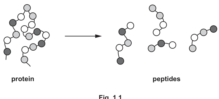
Fig. 1.1
Egg albumen (egg white) contains a high proportion of protein.
10% albumen solution is a cloudy-white colour. This becomes colourless when pepsin is added to the 10% albumen solution.
A student used a colorimeter to follow the progress of the hydrolysis of protein by pepsin.
The student used a blue filter in the colorimeter.
Outline one other step the student should carry out to prepare the colorimeter so that correct measurements of absorbance can be obtained.
Answer
Set the colorimeter to zero absorbance using a blank (a colorimeter tube containing the pH 2.0 buffer and water but no albumen and no pepsin).
Calibrate the colorimeter using a blank to set the absorbance to zero.
Background Concept
A colorimeter measures the absorbance of light by a coloured solution at a particular wavelength, selected by a coloured filter. The filter is chosen so that the solution absorbs strongly at that wavelength, giving a measurable reading. Before any measurements are taken, the instrument must be calibrated against a 'blank' — a cuvette containing everything the sample will contain except the substance being measured (e.g., buffer plus water, no albumen, no pepsin). The blank is placed in the colorimeter and the absorbance is set to zero, so that subsequent readings represent the absorbance due to the substance of interest only.
Understanding the Question
The student is measuring how the absorbance of an albumen–pepsin mixture changes over time as pepsin hydrolyses the cloudy protein into soluble peptides. A blue filter has already been selected. The question asks for one other preparation step so that absorbance readings are 'correct' — i.e. reflect only the absorbance due to the albumen, not background absorbance from the cuvette and the buffer.
Approach
Identify what is in the sample tube that is not the protein of interest — the cuvette walls, the buffer, and any water used to make up the volume. A blank cuvette containing exactly the buffer (and water) but no albumen and no pepsin is used to compensate for these. Insert the blank and adjust the absorbance to zero.
Step-by-Step Reasoning
- The student must compensate for any absorbance of the cuvette and the pH 2.0 buffer solution alone.
- A 'blank' cuvette is prepared containing pH 2.0 buffer (and water) but no albumen and no pepsin.
- The blank is placed in the colorimeter and the absorbance is set to zero.
- This ensures that every subsequent reading reflects only the absorbance of the albumen in the sample.
- Without this step, every reading would be offset by background absorbance, making the calculated rate of change inaccurate.
Key Takeaways
- A colorimeter must be zeroed with a blank before measurements are taken.
- The blank contains everything in the sample except the substance being measured.
- The chosen filter is one preparation step; zeroing the instrument is the other essential step.
Common Mistakes
- Stating 'turn the colorimeter on' — the question says the filter has already been chosen, and trivial answers are not credited.
- Saying 'use water as the blank' — the buffer may absorb slightly at the chosen wavelength, so the blank should match the sample's matrix.
- Failing to state the purpose of the blank (to set the absorbance to zero).
Things to Be Careful About
- The mark scheme allows two equivalent answers: 'calibrate the colorimeter' or 'use a blank to set absorbance to zero'. The second phrasing is more precise and is the safer one to write.
After preparing the colorimeter, the student:
- made a pH 2.0 albumen solution by mixing of 10% albumen solution with of pH 2.0 buffer solution
- added of the pH 2.0 albumen solution to a colorimeter tube
- added a small volume of pepsin solution to the colorimeter tube
- immediately placed the colorimeter tube in the colorimeter
- recorded the absorbance of the mixture every 20 seconds for 5 minutes
- calculated the rate of change in absorbance as a measure of the rate of protein hydrolysis.
The results are shown in Fig. 1.2.
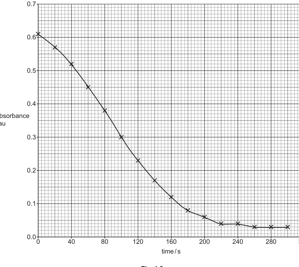
Fig. 1.2
Use Fig. 1.2 to calculate the rate of change in absorbance at pH 2.0 between 40 s and 120 s.
Show your working and include appropriate units.
rate of change in absorbance at pH 2.0 = ______
Working
Reading from Fig. 1.2:
- At : absorbance
- At : absorbance
Answer
0.0036 au s⁻¹
Background Concept
Rate of change of a quantity is calculated as the change in that quantity divided by the change in time. Graphically, it is the gradient of a line or curve. For a smooth curve, the average rate over an interval can be found by reading the y-values at the two endpoints and dividing the difference by the time interval — this is the chord (or secant) gradient over that interval.
In this experiment, the absorbance of the cloudy albumen solution decreases as pepsin hydrolyses the protein into smaller, soluble peptides; a faster decrease in absorbance means a faster rate of protein hydrolysis.
Understanding the Question
Fig. 1.2 plots absorbance (au) against time (s) at pH 2.0. The question asks for the rate of change in absorbance between 40 s and 120 s, with appropriate units. Three marks are available: one for the correct final number, one for the working, and one for the unit.
Approach
- Read the absorbance at from the graph.
- Read the absorbance at from the graph.
- Subtract to find the change in absorbance.
- Subtract the times to find the time interval.
- Divide to find the rate of change.
- Quote the value with the unit .
Step-by-Step Reasoning
Reading from Fig. 1.2:
- At the data point lies just above the 0.5 gridline, so absorbance .
- At the data point lies between 0.2 and 0.3, closer to 0.2, so absorbance .
Change in absorbance:
Time interval:
Rate of change:
The mark scheme accepts or as the final answer. The unit is required for the third mark.
The rate is technically negative (absorbance decreases), but the question asks for the rate of change, and the mark scheme expects the magnitude as a positive number with the unit .
Key Takeaways
- Rate of change on a graph.
- The unit of rate of change of absorbance is absorbance units per unit time, written .
- Reading graphs accurately, showing the working, and including units are all essential for full marks.
Common Mistakes
- Forgetting the unit (the third mark is for the unit alone).
- Using the wrong points (e.g., and ) — this would still score the working mark but gives a less precise average rate.
- Writing a negative number — the convention here is to give the magnitude.
- Failing to show the substitution, losing the working mark.
Things to Be Careful About
- The mark scheme awards 1 mark for the correct final number, 1 mark for the working, and 1 mark for the unit. All three are required for full marks.
- The exact value read from the graph may differ slightly (e.g., or at ); the mark scheme accepts a small range. Use and for consistency with the official answer.
The student decided to investigate the effect of pH on the rate of protein hydrolysis by pepsin.
From the internet the student found out that pepsin is inactive at pH 6.5 and above.
The student was provided with a colorimeter and standard laboratory apparatus.
Describe a method that the student could use to investigate the effect of pH on the rate of protein hydrolysis by pepsin and to determine the optimum pH of pepsin.
Your method should be set out in a logical order and be detailed enough to allow another person to follow it.
Details of how to prepare and use the colorimeter should not be included.
Variables
- Independent variable: pH of the buffer (varied from pH 0 to pH 6.5).
- Dependent variable: rate of change in absorbance (a measure of the rate of protein hydrolysis), in .
- Controlled variables: concentration and volume of pepsin, concentration and volume of albumen, temperature, time interval between readings.
Method
- Prepare at least 5 buffer solutions of stated pH values between pH 0 and pH 6.5 (e.g. pH 1, 2, 3, 4, 5 and 6).
- For each pH, mix of albumen solution with of the pH buffer to give a pH-albumen mixture.
- Place the pH-albumen mixtures and the pepsin solution in a water bath at a stated constant temperature (e.g. ) and leave to equilibrate for 5 minutes.
- Add the same volume (e.g. ) of pepsin solution of the same concentration (e.g. ) to each pH-albumen mixture. Mix and immediately transfer to a colorimeter tube.
- Record the absorbance at intervals for 5 minutes and calculate the rate of change in absorbance (\Deltaabsorbance / \Deltat) for each pH.
- Repeat each pH at least 3 times and calculate a mean rate.
- Plot a graph of mean rate (y-axis) against pH (x-axis) and identify the optimum pH (the pH giving the highest mean rate).
- Repeat the experiment with smaller pH intervals (e.g. every pH unit) around the apparent optimum to determine the optimum more precisely.
Safety
- Hazard: acidic pH buffers (especially at very low pH, e.g. pH 0–2) are corrosive/irritant.
- Risk: skin and eye damage on contact.
- Precaution: wear gloves and safety goggles; wash hands after handling.
See working — a full method covering pH range, controlled variables, mixing, absorbance measurement, replication, optimum identification, and safety.
Background Concept
Enzyme activity is strongly affected by pH. Each enzyme has an optimum pH at which its active site has the correct shape and charge to bind substrate; moving away from the optimum in either direction decreases the rate. At extremes of pH, the enzyme denatures (its tertiary structure is irreversibly disrupted) and activity falls to zero. Pepsin is a protease secreted by the stomach lining and works in acidic conditions; its optimum pH is around 2.0, and it is denatured (inactive) at pH 6.5 and above.
The colorimeter assay used here works because cloudy albumen scatters light; as pepsin hydrolyses the protein into soluble peptides, the solution becomes clearer and the absorbance decreases. The rate of decrease in absorbance is therefore proportional to the rate of protein hydrolysis.
Understanding the Question
The student has been told that pepsin is inactive at pH 6.5 and above. The question asks the student to describe a method to investigate the effect of pH on the rate of protein hydrolysis by pepsin and to determine the optimum pH. The method must be detailed enough for another person to follow, and must exclude colorimeter preparation (which was covered in (a)(i)).
Approach
A good experimental plan should:
- State the independent variable (pH) and the range of values to test.
- State the dependent variable (rate of change in absorbance, in ).
- State the key variables to control (concentration and volume of pepsin, concentration and volume of albumen, temperature).
- Describe the procedure in a logical, step-by-step order, with stated volumes, concentrations and temperatures.
- Include replication (at least 3 repeats per pH) and calculation of a mean.
- Identify the optimum pH from the data (graph of mean rate vs pH).
- Refine the estimate by repeating with smaller pH intervals around the optimum.
- Include a safety point with a named hazard, a specific risk, and a precaution.
Step-by-Step Reasoning
The mark scheme awards up to 10 marks, of which the candidate needs any 7. The marks are distributed across:
- Preparing at least 5 pH buffers (between pH 0 and 6.5) with stated values.
- Using the same concentration/volume of pepsin.
- Controlling temperature (e.g. water bath at a stated temperature).
- Equilibrating all solutions to the same temperature before mixing.
- Mixing pepsin with the pH/albumen solution.
- Measuring absorbance at set time intervals.
- Using at least 3 replicates and calculating a mean rate.
- Identifying the optimum pH from the data.
- Repeating with smaller pH intervals around the optimum.
- Safety: hazard + risk + precaution.
A good plan is a numbered list, written in a logical order, with stated volumes, concentrations, and temperatures wherever possible. Vague statements (e.g. 'control the temperature') without a specific value lose the precision mark.
Key Takeaways
- A planning question is structured: identify variables, control them, vary the independent variable, replicate, and analyse.
- 'Determine the optimum pH' means the experiment must cover a range of pH values and the data must be plotted to find the maximum rate; the estimate is then refined with smaller pH intervals.
- Safety is not optional in a plan — a hazard, a risk, and a precaution are required.
Common Mistakes
- Vague variable control ('use the same amount of pepsin' without a stated volume or concentration).
- Failing to state a temperature or to describe how it is controlled (water bath is the standard answer).
- Not including replicates or a mean.
- Omitting safety or giving an incomplete safety statement (e.g. only a hazard, no risk and no precaution).
- Describing how to use the colorimeter (the question explicitly says not to include this).
- Using too few pH values (e.g. only 2 or 3) — the mark scheme requires at least 5 across the range.
- Forgetting to state how the optimum is identified from the data (graph of rate vs pH).
Things to Be Careful About
- The mark scheme explicitly excludes colorimeter details — the candidate should focus on the experimental design around pH, not on the colorimeter.
- The pH range should span pH 0 to 6.5 because pepsin is inactive at and above pH 6.5, and the student needs to see this decline.
- 'Equilibrate' is the precise word that earns the temperature-equilibration mark — it means to bring all solutions to the same temperature before mixing.
- The safety point requires three components: a named hazard, the specific risk, and a plausible precaution.
Complete the sketch graph in Fig. 1.3 to predict the effect of pH on the rate of protein hydrolysis by pepsin.
Include a label for the y-axis in your answer.
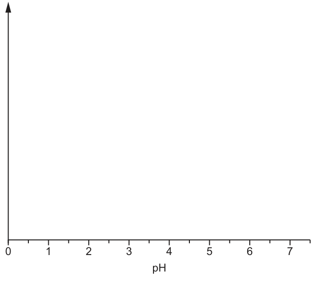
Fig. 1.3
Answer
The y-axis is labelled rate of protein hydrolysis / . The curve starts at a low value at pH 0, rises to a peak at the optimum pH (around pH 2), and then decreases steadily, reaching approximately 0 by pH 6.5 (consistent with pepsin being inactive at pH 6.5 and above).
Y-axis: 'rate of protein hydrolysis / au s⁻¹'; bell-shaped curve with peak at pH 2 and falling to ~0 by pH 6.5.
Background Concept
Enzyme rate vs pH curves are typically bell-shaped with a clear optimum. At the optimum pH, the active site has the correct shape and charge to bind substrate; at pH values above or below the optimum, ionisation of active-site residues (or of the substrate) is altered, reducing activity. At extremes of pH, the enzyme denatures and activity falls to zero. For pepsin, the optimum pH is around 2.0, matching the acidic environment of the stomach. The stem tells us pepsin is inactive at pH 6.5 and above.
Understanding the Question
The question provides an empty graph with pH (0 to 7) on the x-axis and an unlabelled y-axis arrow. The candidate is asked to predict the shape of the rate vs pH curve and to provide a y-axis label. The prediction should be consistent with pepsin's known properties (optimum near pH 2, inactive at pH 6.5 and above).
Approach
Draw a curve that:
- Starts at a low value at pH 0 (some activity, but not maximum).
- Rises to a peak at around pH 2 (the optimum).
- Decreases steadily as pH rises above 2.
- Reaches 0 (or near 0) by pH 6.5, reflecting that pepsin is inactive above this pH.
- Label the y-axis 'rate of protein hydrolysis / ' (the unit used in (a)(ii)).
Step-by-Step Reasoning
At pH 0, conditions are too acidic for the active site to function optimally — the active site is distorted and activity is low. As pH rises towards 2, ionisation of the active-site residues becomes favourable and activity increases. At pH 2 (the optimum), the active site is the correct shape and charge for maximum rate. Above pH 2, the active site gradually loses its functional ionisation state and activity falls. By pH 6.5, the enzyme is fully inactive (as stated in the stem), so the rate is 0.
The curve should not be perfectly symmetrical: pepsin's curve typically drops more gradually on the high-pH side. The exact shape is not critical — the key features (low start, peak around pH 2, drop to 0 by pH 6.5–7) are what earn the mark.
Key Takeaways
- An enzyme rate vs pH curve is bell-shaped with an optimum.
- The optimum pH for pepsin is around 2, reflecting its role in the stomach.
- At pH values far from the optimum, the enzyme is denatured and activity is 0.
- Sketch graphs need a labelled y-axis and a clear, appropriately shaped curve.
Common Mistakes
- Drawing a straight line or a continuously increasing/decreasing curve (not a peak).
- Placing the optimum at the wrong pH (e.g. pH 7).
- Not labelling the y-axis.
- Drawing a curve that does not reach 0 at pH 6.5 (the stem explicitly says pepsin is inactive above pH 6.5).
Things to Be Careful About
- The y-axis label must match the variable being plotted (rate of protein hydrolysis) and include the correct unit ().
- The x-axis is already labelled pH, so the candidate only needs to add the y-axis label and the curve.
- The curve should be smooth and continuous — not a series of straight-line segments.
Laryngopharyngeal reflux (LPR) is a disease that occurs when gastric juice from the stomach moves up the oesophagus and into the larynx, as shown in Fig. 1.4.
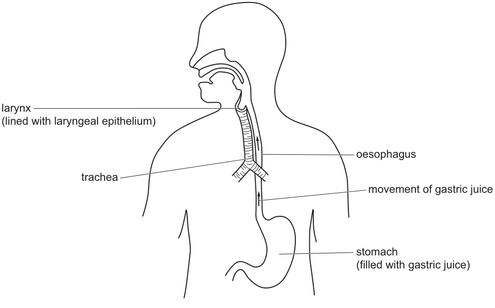
Fig. 1.4
Gastric juice can damage the laryngeal epithelium. Gastric juice contains hydrochloric acid and pepsin.
Some scientists identified a reduction in the quantity of two proteins, CA3 and Sep70, present in the laryngeal epithelium of people with LPR.
The scientists obtained 6 sections of mammalian laryngeal epithelium to investigate how different test conditions affect the quantity of CA3 and Sep70 in the laryngeal epithelium.
Each section of laryngeal epithelium was exposed to different test conditions for 20 minutes, as shown in Table 1.1.
Pepsin is inactive in the presence of the inhibitor, pepstatin.
Table 1.1
| treatment used | test condition 1 | test condition 2 | test condition 3 | test condition 4 | test condition 5 | test condition 6 |
|---|---|---|---|---|---|---|
| pepsin | yes | yes | yes | yes | no | no |
| pepstatin (inhibitor) | no | no | yes | yes | yes | yes |
| pH buffer | 7.4 | 4.0 | 7.4 | 4.0 | 7.4 | 4.0 |
Proteins were then extracted from the sections of laryngeal epithelium. The proteins were separated using electrophoresis. CA3 and Sep70 were identified using fluorescent antibodies.
Fig. 1.5 shows the results of the protein electrophoresis.
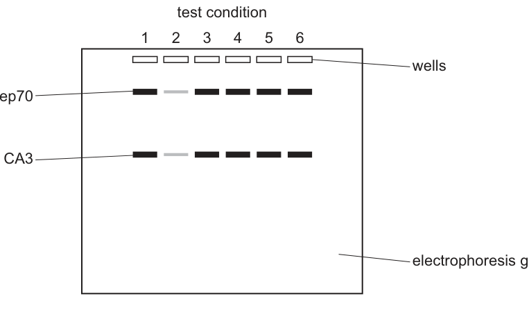
Fig. 1.5
Use Table 1.1 and Fig. 1.5 to state the conclusions that can be made from the results of the protein electrophoresis.
Answer
- Test condition 2 (pepsin present, no pepstatin, pH 4.0) caused a large decrease in the quantity of both CA3 and Sep70 — only this lane shows faint bands.
- Acid alone (pH 4.0) without active pepsin does not change the quantity of CA3 or Sep70 (test condition 4: pepstatin-inhibited pepsin at pH 4.0 still shows thick bands).
- CA3 is smaller than Sep70 (or Sep70 is larger than CA3) — the CA3 band has migrated further through the gel from the well than the Sep70 band.
Active pepsin at pH 4.0 hydrolyses both CA3 and Sep70; acid alone has no effect; CA3 is smaller than Sep70.
Background Concept
Gel electrophoresis separates proteins by size. Proteins are loaded into wells at one end of a gel, and an electric current is applied. The proteins migrate through the gel; smaller proteins move faster and travel further, so they appear further from the well. The amount of protein at a given position can be estimated by the intensity (thickness and darkness) of the band.
In this experiment, scientists exposed sections of mammalian laryngeal epithelium to different combinations of pepsin, an inhibitor (pepstatin), and pH. The pH buffer determines whether pepsin is active (pepsin is active at acidic pH, around pH 2, and inactive at pH 7.4). Pepstatin inhibits pepsin regardless of pH. The proteins CA3 and Sep70 are then extracted and run on a gel to see how much of each remains.
Understanding the Question
Table 1.1 specifies six test conditions:
- Pepsin, no inhibitor, pH 7.4 (pepsin inactive due to pH).
- Pepsin, no inhibitor, pH 4.0 (pepsin ACTIVE).
- Pepsin + pepstatin, pH 7.4 (pepsin inactive due to both pH and inhibitor).
- Pepsin + pepstatin, pH 4.0 (pepsin would be active at this pH but pepstatin inhibits it).
- No pepsin, pepstatin, pH 7.4 (no pepsin present).
- No pepsin, pepstatin, pH 4.0 (no pepsin present).
Fig. 1.5 shows the gel: in test condition 2, the bands for both CA3 and Sep70 are faint (much less protein); in all other conditions, the bands are thick and dark (full amount of protein).
Approach
Compare each lane in Fig. 1.5 with the corresponding conditions in Table 1.1 to identify which combination causes the reduction in protein bands. The single condition that produces faint bands is condition 2 — the only one with active pepsin (no pepstatin, acidic pH 4.0). All other conditions either lack pepsin or have pepstatin-inhibited pepsin.
Also compare band positions: the CA3 band is further from the wells than the Sep70 band, so CA3 is the smaller protein.
Step-by-Step Reasoning
Test condition 2: faint bands for both CA3 and Sep70 → active pepsin at pH 4.0 hydrolyses (reduces) both proteins.
Test condition 4: thick bands for both proteins → acid alone (pH 4.0) without active pepsin does NOT reduce CA3 or Sep70.
Test condition 1: thick bands → pepsin at pH 7.4 is inactive, so it does not reduce the proteins (consistent with condition 2 being the only one that does).
Test conditions 3, 5, 6: thick bands → no pepsin, or inhibited pepsin, or inactive pepsin; proteins remain.
Band positions: CA3 bands are further from the wells than Sep70 bands, meaning CA3 is the smaller protein and Sep70 is larger.
Three possible conclusions (any 2 for 2 marks):
- Test condition 2 (active pepsin at pH 4.0) decreases both CA3 and Sep70.
- Acid alone (without active pepsin) does not change CA3 or Sep70.
- CA3 is smaller than Sep70 (or Sep70 is larger than CA3).
Key Takeaways
- Gel electrophoresis separates proteins by size; smaller proteins travel further.
- The intensity of a band reflects the quantity of that protein.
- Comparing lanes with different treatments identifies the cause of an effect.
- A valid conclusion must be supported by the data: here, the only condition that produces faint bands is condition 2, so active pepsin at acidic pH is the cause.
Common Mistakes
- Saying 'pepsin breaks down the proteins' without specifying that it must be ACTIVE (i.e. pH 4.0 with no inhibitor).
- Concluding that acid alone causes the effect (it does not — condition 4 with acid and inhibited pepsin shows thick bands).
- Missing the band position observation (CA3 is smaller than Sep70).
- Misidentifying the direction of electrophoresis (smaller = further from well, not closer).
Things to Be Careful About
- The mark scheme allows three possible conclusions; the candidate only needs 2 for full marks.
- 'Decreases' or 'hydrolyses' are both acceptable verbs.
- The mark scheme explicitly allows the observation that CA3 is smaller (or Sep70 larger) — the candidate should use 'mass', 'size', or 'molecular weight' terminology.
The results of this investigation were published in a scientific paper.
A student who read the scientific paper concluded that pepsin causes damage to the laryngeal epithelium in people with LPR.
Suggest why the results of this investigation might not support this conclusion.
Answer
Any two of:
- The investigation was not repeated — only one section of laryngeal epithelium was used for each condition, so the results may not be reliable / reproducible.
- The species of mammal used is not stated — the results may not apply to humans with LPR.
- The investigation was carried out in the laboratory (in vitro) on isolated epithelium sections, not in a person with LPR, so the conditions do not fully reflect what happens in the disease.
- A reduction in the quantity of CA3 and Sep70 may not necessarily cause damage to the laryngeal epithelium (a reduction does not prove that these proteins are the cause of the damage).
See working — the study was not repeated, the species is unknown, the work is in vitro on isolated tissue, and a protein reduction does not prove causation of damage.
Background Concept
A scientific conclusion must be supported by the experimental data and by the experimental design. Limitations of an investigation can weaken a conclusion even if the data themselves are accurate. Common limitations include: small sample size (no replicates), use of a different species (results may not generalise), in vitro rather than in vivo conditions, and not establishing causation (only correlation).
Understanding the Question
A student reading the paper concluded that 'pepsin causes damage to the laryngeal epithelium in people with LPR'. The question asks the exam candidate to suggest reasons why the results of the investigation might not support this conclusion. The candidate must identify weaknesses in the experimental design or in the logical chain from data to conclusion — not simply state that the data are wrong.
Approach
Consider each link in the chain:
- The data show that active pepsin (with acid) reduces CA3 and Sep70 in isolated laryngeal epithelium sections.
- The conclusion is that pepsin causes damage to the laryngeal epithelium in people with LPR.
- What could break this chain?
- The data are from isolated sections, not from a living person (in vitro vs in vivo).
- Only one section per condition — not replicated, so the result may not be reliable.
- The species of mammal is not stated — the sections may not be from humans.
- Even if CA3 and Sep70 are reduced, that may not cause the actual tissue damage seen in LPR (the reduction could be a consequence, not a cause, of damage; or a different protein may be responsible).
Step-by-Step Reasoning
The mark scheme awards marks for any 2 of the following:
- Pepsin only causes a reduction in CA3 and Sep70 if acid is also present — so the role of pepsin alone in LPR is not established (though the question is more about whether the investigation supports the broad conclusion that pepsin causes damage in LPR; in LPR both are present, but the experimental design still has the limitations below).
- The investigation was not repeated — only one section per condition, so the results may not be reproducible.
- No information about the species of mammal — the results may not apply to humans.
- The investigation was carried out in the laboratory, not in a person with LPR, so the conditions may not reflect what happens in the disease.
- A reduction in CA3 and Sep70 may not cause damage to the laryngeal epithelium (the causal link is not established).
The best answers will identify that the investigation is in vitro and not in a person, that the species is not specified, that there is no replication, and that reduced proteins do not necessarily mean damage.
Key Takeaways
- Drawing conclusions from experimental data requires considering the limitations of the data.
- In vitro results do not necessarily apply to whole organisms or to disease states in vivo.
- Replication and species information are basic requirements for valid conclusions.
- A change in molecular quantity (protein level) is not the same as a change in tissue function or damage.
Common Mistakes
- Stating 'human error' or 'inaccurate results' — these are not specific limitations of this investigation.
- Failing to identify that the experiment was in vitro (a critical limitation).
- Stating that the data prove the conclusion is wrong — the question asks why the data might not support the conclusion; they could still be consistent with it, just not definitive.
- Ignoring the species issue.
- Confusing 'no replication' with 'not enough data' — the specific point is that only one section was used per condition.
Things to Be Careful About
- The mark scheme accepts four different limitations; the candidate only needs 2 for full marks.
- The candidate should not say 'the experiment shows pepsin doesn't cause damage' — the data actually show that active pepsin does reduce these proteins, but the question is about whether this supports the conclusion that pepsin causes LPR damage in people.
- Use precise scientific language: 'in vitro' (not 'in a test tube', though this is acceptable); 'replicated' (not 'repeated' as a vague term); 'species' (not 'type of animal' if possible).
Golden orb weaver spiders, Nephila pilipes, are found in East Asia, South-east Asia and Australia. They are active in the day and at night. Golden orb weaver spiders build webs in trees and shrubs to catch different species of insects for food.
All female golden orb weaver spiders are black with yellow spots on their legs and body. Biologists think that this adaptation evolved due to natural selection. Spiders with yellow spots may be able to attract more insects to their webs.
Fig. 2.1 shows a female golden orb weaver spider sitting on a web.
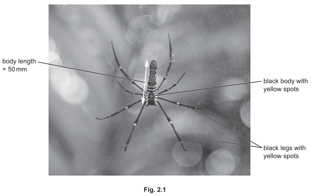
Fig. 2.1
Some biologists visited a forest in East Asia in July 2008. The biologists found five webs that were approximately the same size. Each web belonged to a female golden orb weaver spider.
The biologists decided to investigate how the colour and pattern of spots on the spiders affect the number of insects attracted per hour to each web (insect attraction rate).
The biologists made two-dimensional (2D) models of spiders, as shown in Table 2.1.
Table 2.1
| model | description | diagram |
|---|---|---|
| A | • black body with yellow spots • black legs with yellow spots • same colour and pattern of spots as golden orb weaver spiders | |
| B | • black body with blue spots • black legs with blue spots • same pattern of spots as golden orb weaver spiders | |
| C | • black body with large yellow spot • black legs • total area of yellow colour is the same as model A | |
| D | • yellow body • yellow legs | |
| E | • black body • black legs |
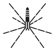
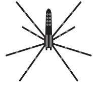



At the first web, the biologists:
- removed the living golden orb weaver spider from the web
- placed model A in the centre of the web
- placed a video camera 1 m from the web
- filmed the web and model for 6 hours
- recorded an insect attraction event whenever an insect flew towards the model, touched the model, or touched the web
- calculated the insect attraction rate of model A.
The procedure was repeated by placing models B, C, D and E on the four other webs.
The whole investigation was repeated 25 times, and a mean insect attraction rate for each model was calculated.
Answer
Number of insect attraction events (in 6 hours).
Number of insect attraction events (in 6 hours)
Background Concept
A dependent variable is the variable that is measured in an experiment — the response to whatever is being deliberately changed. The independent variable is the variable that the experimenter changes on purpose. In any controlled comparison, only the independent variable should vary between treatment groups; the dependent variable is the measured outcome used to detect any effect.
Understanding the Question
The biologists have built five 2-D models that differ in colour and in the pattern of the yellow spots (Table 2.1). They place one model in the centre of a web, film for 6 hours and record every insect that flies towards, touches the model or touches the web. They then repeat the procedure 25 times and calculate a mean.
We are asked to identify the dependent variable — the quantity that is measured as the response.
Approach
Look at what the biologists actually record during the 6-hour filming. Whatever they count is the dependent variable. The five model types form the independent variable (the variable that is changed), so the answer must be the response that is measured when each model is used.
Step-by-Step Reasoning
- The procedure records "an insect attraction event whenever an insect flew towards the model, touched the model, or touched the web".
- The raw measurement is therefore the count of insect attraction events in the 6-hour filming window.
- The mean rate (insects per hour) is then calculated from these counts, but the underlying measurement — what actually depends on the model being tested — is the number of events.
Key Takeaways
- The dependent variable is the response measured, not the rate calculated from it.
- Read the procedure carefully: "recorded an insect attraction event whenever…" tells you that the measurement is the count of events.
Common Mistakes
- Confusing the independent variable (which model is on the web) with the dependent variable.
- Writing the rate (insects h⁻¹) instead of the count of events — the rate is a derived value, not the raw measurement that the mark scheme rewards.
Things to Be Careful About
- "Number of insect attraction events" is the precise wording the mark scheme requires; "insect attraction rate" or a bare "number of insects" is too vague.
The pattern of spots on models A and B was the same as the pattern of spots on female golden orb weaver spiders.
Identify two other variables that the biologists should standardise when making the models for this investigation.
Answer
Any two from:
- size / length of the model (or of the body / legs)
- shape of the model
- material of the model
- thickness / mass / weight / density of the model
- size of the spots (on models A and B)
- (models are) odourless
- yellow colour / shade / tone of the yellow paint
- light absorption / reflection of the models
Any two from: size of model, shape of model, material of model, mass/weight, size of spots, odourless, yellow colour shade, light reflection
Background Concept
In a fair test, only the independent variable is allowed to differ between treatment groups. Every other variable that could plausibly affect the response must be standardised (kept the same), so that any difference in the dependent variable can be attributed to the independent variable and not to a confounding factor.
Understanding the Question
We are told that the pattern of spots is the same on models A and B. The investigation is testing whether colour and pattern of spots affect insect attraction. Everything else about the models must therefore be identical, or a difference in attraction rate could be caused by something other than colour/pattern.
Approach
List physical and sensory properties of the models that could affect how many insects are attracted. Choose two that should be standardised so that any remaining difference in attraction rate is due only to colour/pattern.
Step-by-Step Reasoning
Possible variables to standardise (any two are credited):
- Size / length of the model, body or legs — a larger silhouette is more visible to insects, so all models must be the same size.
- Shape of the model — a different outline (e.g. a more compact body) could change how visible the model is.
- Material of the model — paper, plastic, card and fabric all reflect light differently and would change how the model appears.
- Mass / weight / thickness / density of the model — affects how the model sits in the web and how the web moves in air currents, both of which could affect insects.
- Size of the spots (on A and B) — must be the same so that pattern alone (not spot size) is what differs.
- Odour — any smell from the model could itself attract or repel insects; models must be odourless.
- Yellow colour / shade / tone of the yellow paint — must be the same yellow across models so that differences are due to the area or pattern of yellow, not the shade.
- Light absorption / reflection of the model — how the model reflects sunlight affects how visible it is to flying insects.
Key Takeaways
- Standardising means keeping all non-test variables identical across treatments.
- A confound is anything else that could affect the response — here, anything about the models that could change how visible or attractive they are to insects.
Common Mistakes
- Listing the variable being tested (colour/pattern) — that is the independent variable and is deliberately not standardised.
- Vague answers such as "everything else the same" — the mark scheme requires a specific, named variable.
- Listing variables that cannot plausibly affect insects (e.g. "the colour of the table they were made on").
Things to Be Careful About
- The wording matters: "size" alone is fine; "bigger" or "small" on its own is not specific enough.
- "Material" and "odourless" are different points — choose whichever best fits the mark.
Answer
(Measure the insect attraction rate of) a web with no model on it.
A web with no model
Background Concept
A control is a treatment in which the independent variable is absent (or held at a baseline), so that the experimenter can measure what happens without the experimental intervention. Comparing treatments to the control reveals the effect of the intervention itself, rather than simply describing the treatment response in isolation.
Understanding the Question
The investigation tests five different spider models. The question asks what would serve as a suitable control. We need a treatment that lacks the variable being tested — here, the presence (and appearance) of a spider model — but is otherwise identical to the experimental procedure.
Approach
The most natural control is the web without any model at all. The filming, the web, the camera, the 6-hour period and the 25 repeats can all be reproduced exactly; only the model is missing. This shows the baseline insect attraction rate to a bare web, against which each model can be compared.
Step-by-Step Reasoning
- All five models are experimental treatments — each one tests a particular colour/pattern combination.
- A control must be the same web under the same conditions but with the independent variable (the model) removed.
- The control therefore consists of filming an empty web (no model) for 6 hours and counting the insect attraction events, using the same procedure and replication.
- The mean attraction rate of the bare web can then be compared against the rates for models A–E, so that the additional attraction due to the model (and its appearance) can be quantified.
Key Takeaways
- A control is the "no-treatment" baseline, reproduced as closely as possible to the experimental procedure.
- Without a control, an attraction rate of 0.21 insects h⁻¹ (model A) cannot be distinguished from the rate that the web alone would produce.
Common Mistakes
- Choosing one of the existing models (A, B, C, D or E) as the control — these are all experimental treatments, not controls.
- Suggesting a "control web in a different forest" — this introduces a new variable (location) instead of removing the model.
Things to Be Careful About
- The control must be a bare web in the same forest under the same conditions, so that any difference in insect attraction can be attributed to the model rather than to changes in weather, location, time of day, etc.
Fig. 2.2 shows the mean insect attraction rates for the five models. The error bars show one standard error (SE).
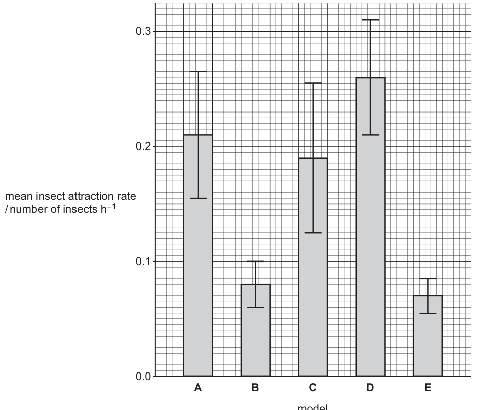
Fig. 2.2
Use the information shown in Table 2.1 and Fig. 2.2 to discuss the conclusions that can be made about the effect of colour and pattern of spots on the models on insect attraction rates.
Answer
- The yellow models (A, C, D) have higher mean insect attraction rates than the non-yellow models (B, E).
- Colour (yellow vs not yellow) appears to be the dominant factor; the pattern of the spots (compare A with C, or A with B) has much less effect than the presence of yellow.
- The standard error bars of the yellow models (A, C, D) do not overlap with those of the non-yellow models (B, E), so the difference in mean attraction rate between yellow and non-yellow models is likely to be statistically significant.
- The standard error bars of A, C and D overlap with each other (and those of B and E overlap with each other), so the differences between models of the same colour are unlikely to be statistically significant.
- Data quote: e.g. model D (all yellow) had a mean rate of insects h⁻¹, while model E (all black) had a mean rate of insects h⁻¹.
Yellow colour, not the pattern of spots, significantly increases the mean insect attraction rate; the pattern of spots has little additional effect.
Background Concept
When a mean is plotted with standard error (SE) bars, the bars give a visual impression of how precisely the mean has been estimated. A useful — though not absolute — rule of thumb is that if the SE bars of two means do not overlap, the difference is likely to be statistically significant, whereas overlapping SE bars suggest the difference is unlikely to be statistically significant. (A formal test, such as a t-test, is needed to confirm.)
The standard error itself is the standard deviation of the sample means; it is calculated as
where is the standard deviation and is the sample size. It is not a measure of the spread of the raw data — that is the standard deviation.
Understanding the Question
Fig. 2.2 is a bar chart of the mean insect attraction rate for each of the five models, with SE bars above and below each mean. We are asked to discuss what the data show about the effect of colour and pattern of the spots on insect attraction. A good answer must (i) describe the effect of colour, (ii) describe the effect of pattern, (iii) use the error bars to make a statement about likely significance, and (iv) support the argument with quoted data.
Reading from Fig. 2.2 (approximate values):
- Model A (black body + legs, small yellow spots): mean ≈ 0.21 insects h⁻¹; SE bars ≈ 0.15 – 0.27
- Model B (black body + legs, small blue spots): mean ≈ 0.08 insects h⁻¹; SE bars ≈ 0.06 – 0.10
- Model C (black body + legs, one large yellow spot): mean ≈ 0.19 insects h⁻¹; SE bars ≈ 0.13 – 0.25
- Model D (all yellow body + legs): mean ≈ 0.26 insects h⁻¹; SE bars ≈ 0.21 – 0.31
- Model E (all black body + legs): mean ≈ 0.07 insects h⁻¹; SE bars ≈ 0.05 – 0.08
Approach
- Sort the models by colour: yellow present (A, C, D) vs no yellow (B, E). Compare their means.
- Within the yellow group, compare A (many small spots) vs C (one large spot) vs D (all yellow) — this tests the effect of pattern.
- Within the non-yellow group, compare B (with blue spots) vs E (plain black) — the blue spots are a different colour but the pattern is the same as A.
- Use SE bar overlap to make statements about likely statistical significance.
- Quote at least one mean with units (e.g. model D vs model E) to support the conclusion.
Step-by-Step Reasoning
- Effect of colour: the three models with yellow (A, C, D) have means of ≈ 0.21, 0.19 and 0.26 insects h⁻¹. The two non-yellow models (B, E) have means of ≈ 0.08 and 0.07 insects h⁻¹. The yellow models clearly attract more insects, so colour (yellow vs not yellow) has a large effect.
- Effect of pattern: within the yellow group, the three models have very similar means (0.19 – 0.26 insects h⁻¹) and their SE bars all overlap. This means the precise distribution of yellow (small spots, one big spot, or all yellow) makes little difference — colour is the dominant factor, not the pattern of the spots.
- Statistical significance (colour): the SE bars of the yellow models (lower end ≈ 0.13 – 0.21) lie above the upper ends of the SE bars of the non-yellow models (upper end ≈ 0.08 – 0.10). The bars do not overlap, so the difference between yellow and non-yellow is likely to be statistically significant.
- Statistical significance (pattern): the SE bars of A, C and D all overlap with each other, so the differences between them are unlikely to be statistically significant. The SE bars of B and E also overlap, so the difference between the two non-yellow models is not significant either.
- Data quote: e.g. "model D (all yellow) had a mean of ≈ 0.26 insects h⁻¹ compared with ≈ 0.07 insects h⁻¹ for model E (all black)" — quoting these values, with units, makes the conclusion concrete and supports the argument with evidence from the figure.
Key Takeaways
- A bar chart with SE bars can be read both as a comparison of means and as a rough guide to statistical significance.
- Non-overlap of SE bars is a quick visual proxy for "probably significant"; overlap suggests "probably not significant". A formal test is still needed.
- When a question asks to "discuss", you must consider both factors being tested (here, colour AND pattern) and reach a conclusion about each.
Common Mistakes
- Only describing colour and ignoring pattern (or vice versa) — both must be addressed.
- Reading the y-axis as the standard deviation rather than the standard error, leading to a different (and incorrect) interpretation of the bars.
- Concluding that, because the means are different, the difference must be significant — the SE bars must be examined.
- Forgetting to quote a value with units; the mark scheme requires a data quote to support the argument.
Things to Be Careful About
- The SE bars are ± one SE, not ± 2 SE (≈ 95% CI) and not the standard deviation. They give the precision of the mean, not the spread of the raw data.
- Do not claim that overlap of SE bars is a definitive test — it is only a guide. The question is asking for a discussion using the figure, not for the result of a t-test.
- When quoting a mean, always give the units (insects h⁻¹).
The biologists decided to analyse the data in Fig. 2.2 using -tests.
State a null hypothesis the biologists could make before carrying out the -tests.
Answer
There is no significant difference between the mean insect attraction rates of the (different) models.
There is no significant difference between the mean insect attraction rates of the models
Background Concept
A null hypothesis (H₀) is a statement of "no effect" or "no difference" between the populations being compared. It is the hypothesis that a statistical test is set up to test against. The alternative hypothesis (H₁ or Hₐ) is the opposite — that there is a difference. A null hypothesis must be testable and falsifiable, so that the data can be used to assess whether to reject it.
For a t-test comparing two means, the null hypothesis is that the two population means are equal (any difference observed in the sample is due to random chance).
Understanding the Question
The biologists have mean insect attraction rates for five different models (A–E) and intend to run t-tests. We are asked to state a suitable null hypothesis before carrying out the tests.
Approach
A correct null hypothesis for a t-test comparing means says, in plain words, "there is no significant difference between the means". It does not predict the direction of any difference, and it does not name a specific pair of models (because the t-test is applied to multiple pairs).
Step-by-Step Reasoning
- The variable being compared across the models is the mean insect attraction rate.
- The null hypothesis is the "no difference" statement: any difference between the means is attributed to chance variation between samples.
- It must be written in terms of the populations the samples came from, but the standard CIE phrasing in this context is "there is no significant difference between the mean insect attraction rates of the models".
Key Takeaways
- A null hypothesis is always a statement of "no significant difference" or "no significant effect".
- It should be phrased in terms of the means (here, mean insect attraction rates) because that is what the t-test compares.
- It must be testable by the chosen statistical test.
Common Mistakes
- Phrasing the null hypothesis as a difference that does exist (e.g. "model A attracts more insects than model E") — that is the alternative hypothesis, not the null.
- Naming only two models — the hypothesis should at least be unambiguously written in the form "no significant difference between the means of [pair of models]".
- Forgetting the word "significant"; a bare "no difference between the means" is too absolute because random variation always produces small sample-to-sample differences.
Things to Be Careful About
- The hypothesis must be stated before the data are analysed — a t-test cannot be used to "prove" a hypothesis that was generated by looking at the means in Fig. 2.2.
- Avoid the word "equal" in the formal phrasing unless you specifically mean the population means; the standard CIE phrasing is "no significant difference".
State two reasons why the -test is suitable for analysing the data shown in Fig. 2.2.
Answer
Any two from:
- The data are continuous (number of insects per hour).
- A t-test compares two means.
- The sample size is fewer than 30 (n = 25).
- The data are (assumed to be) normally distributed.
Any two from: data is continuous, comparing two means, fewer than 30 values, normally distributed
Background Concept
The Student's t-test is a statistical test used to compare the means of two samples and decide whether the difference between them is statistically significant. It is appropriate only when certain conditions (assumptions) are met:
- The data are continuous (numerical, on a measurement scale, not counts of categories).
- The samples come from populations that are normally distributed (or, for the t-test specifically, the sampling distribution of the mean is approximately normal — which is true for moderate even if the raw data are not perfectly normal).
- The sample size is small (typically ); for large samples the z-test is used instead.
- The two samples are independent (i.e. no pairing between observations in the two groups).
The t-test produces a t-statistic, which is compared against a critical value (looked up in a table at the chosen significance level, usually , and the appropriate degrees of freedom) to decide whether to reject the null hypothesis.
Understanding the Question
The biologists will run t-tests on the data in Fig. 2.2. We are asked to state two reasons why the t-test is suitable — i.e. two features of the data that match the assumptions of the t-test.
Approach
Look at each of the four standard assumptions of the t-test and decide which of them are met by the data in this investigation. Pick any two to write as the answer.
Step-by-Step Reasoning
- Continuous data: the mean insect attraction rate (insects h⁻¹) is a continuous numerical variable — it can take any value in a range. ✓ This is one reason the t-test is suitable.
- Comparing two means: each t-test compares the mean of one model with the mean of another model. ✓ This matches the test's purpose.
- Sample size < 30: the investigation was repeated 25 times for each model, so , which is less than 30. The t-test is the appropriate test for samples of this size. ✓
- Normally distributed populations: the data are assumed to be drawn from approximately normally distributed populations, which is one of the standard assumptions of the t-test. ✓
Any two of these four points earn the marks.
Key Takeaways
- Choosing a statistical test is a matter of checking the data against the test's assumptions.
- The t-test is the standard small-sample test for comparing two means of continuous data.
- For large samples () the z-test (or a normal-approximation test) is used instead.
Common Mistakes
- Listing reasons that are not actually assumptions of the t-test (e.g. "there are 5 models", "the bars are large").
- Stating only one reason when two are required — the question is worth 2 marks and explicitly asks for two reasons.
- Confusing the t-test with the chi-squared test (which is used for categorical data and observed-vs-expected counts) or with Spearman's rank correlation (used for two variables, not two means).
Things to Be Careful About
- "Data is continuous" is not the same as "data is a count" — insect attraction is a count, but the rate (insects per hour) is continuous.
- "Fewer than 30 values" is specifically about the sample size , not about the number of groups or the number of models.
A student thought that the investigation did not provide enough information about how the colour and pattern of spots on female golden orb weaver spiders help to attract insects to their webs.
Suggest how this investigation could be improved to increase confidence in the results.
Answer
Any two from:
- Repeat the investigation in more than one forest / geographical area.
- Carry out the investigation at different times of the day.
- Carry out the investigation in more than one month / season / year.
- Only count insects that touch the model / web (rather than also counting insects that simply fly towards the model).
- Use more models with different colours / patterns, or use a 3-D model instead of a flat 2-D model.
- Use a (video of a) living spider on the web.
Any two from: more than one forest, different times of day, different months/seasons, only count insects that touch the model/web, more models or 3-D model, use a living spider
Background Concept
Improving the confidence in a result means reducing the impact of confounding variables and increasing the representativeness of the sample. In a field experiment like this one, the main threats to confidence are:
- Local effects — a single forest, a single time of day, a single month or year may give an unrepresentative picture of the general pattern.
- Measurement error — counting insects that simply fly towards a model may overestimate the attraction; the 2-D nature of the models does not mimic the appearance of a real spider.
- Ecological validity — testing models instead of real spiders limits how well the conclusion applies to the real biology of the species.
A good improvement addresses one of these threats directly.
Understanding the Question
A student thinks the investigation is not enough to show how the colour and pattern of spots on real female golden orb weaver spiders help to attract insects. We are asked to suggest two improvements that would increase confidence in the results.
Approach
Think of the threats to confidence listed above and pick two specific, concrete improvements that the biologists could realistically make. Each must be a real change to the design, not a vague statement.
Step-by-Step Reasoning
- More than one forest / geographical area — the result from a single East-Asian forest in July 2008 may not generalise to other regions or to the species as a whole. Repeating the study in several different forests would make the conclusion more widely applicable.
- Different times of day — the species is active both day and night, and insect activity also varies with the time of day. Sampling at multiple times would smooth out this source of variation.
- More than one month / season / year — insect abundance and activity vary with the season; a July-only study may not represent the annual pattern.
- Only count insects that actually touch the model or the web — the current definition of an "insect attraction event" includes insects that merely fly towards the model, which inflates the count. Restricting the count to actual contact would more closely measure the relevant biological outcome (insects being caught).
- More models with different colours / patterns, or 3-D models — a wider range of treatments, or 3-D models, would let the biologists explore the effect of colour and pattern more thoroughly, and the 3-D form would more closely resemble a real spider.
- Use a (video of a) living spider on the web — replacing the model with a real (or filmed) spider would directly test the real organism, rather than a paper model, removing the question of whether the model adequately mimics the appearance of the spider.
Any two of the above earn the marks.
Key Takeaways
- Improvements must be specific and realistic — they should name the variable that would be changed and the reason.
- The most important improvements to a field experiment are usually more replication (more sites, times or seasons) and reducing confounding (better measurement criteria, more realistic test subjects).
Common Mistakes
- Vague answers like "do it again", "take more readings" or "be more accurate" — the mark scheme credits specific, named changes.
- Improvements that are about analysis rather than design (e.g. "use a different statistical test") — the question is about the investigation itself.
- Improvements that introduce a new confound (e.g. "use a different web") rather than addressing the existing threats.
Things to Be Careful About
- Match each improvement to the specific weakness it fixes: more sites fixes "only one location"; only counting contact fixes "over-counted"; using a 3-D model or a real spider fixes "flat paper models may not mimic a real spider".
- The mark scheme requires two distinct improvements; writing the same idea twice in different words earns only one mark.