Biology 9700/52 — October/November 2024

Cambridge A-Level · Planning, Analysis and Evaluation · worked solutions for every part, with the mark scheme

questions

marks

minutes

Topics Planning · Analysis, Conclusions and Evaluation

Q1Medium-HardPlanningAnalysis, Conclusions and Evaluation

In the light-dependent stage of photosynthesis, electrons and hydrogen ions are accepted by the coenzyme NADP, which becomes reduced.

DCPIP is a dye that can act as an electron and hydrogen ion acceptor. The dye is blue when oxidised and colourless when reduced. In laboratory experiments, DCPIP can be used to follow the progress of the light-dependent stage because it can replace NADP as the acceptor molecule for electrons and hydrogen ions, as shown in Fig. 1.1.

Fig. 1.1

The effects of various factors on the light-dependent stage of photosynthesis can be investigated by using suspensions of isolated chloroplasts (chloroplast suspensions) and DCPIP.

A student used DCPIP to investigate the effect of temperature on the rate of the light-dependent stage of photosynthesis in spinach, Spinacia oleracea.

The student prepared a leaf extract to make a stock chloroplast suspension and then carried out a preliminary experiment to determine a suitable concentration of chloroplast suspension to use in the investigation.

To carry out the preliminary experiment, the student followed a set of instructions, steps 1 to 11.

Cut spinach leaves into small pieces and place these pieces in a blender containing ice-cold 10% sucrose solution buffered at pH 7.0.
Turn on the blender for 15 seconds and then filter the extract to remove all the small pieces of leaf.
Place the leaf extract in a centrifuge and spin at low speed.
Pour off the supernatant that contains the chloroplasts. Keep this stock chloroplast suspension ice cold and in the dark.
Prepare 5 different concentrations of the chloroplast suspension using 10% sucrose solution. The percentage concentrations are 10%, 20%, 30%, 40% and 50% of the stock chloroplast suspension.
Wrap 5 flat-bottomed tubes in black plastic film to prevent light entering.
Put $10\ \text{cm}^3$ of each concentration of stock chloroplast suspension into a flat-bottomed tube, and add $1\ \text{cm}^3$ of DCPIP solution to each tube. The chloroplast suspension is now blue-green in colour.
Place 1 of the tubes beneath a light source as shown in Fig. 1.2.

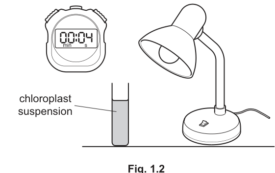
Fig. 1.2

Start a timer. Remove the black plastic film from the tube. Record the time taken for the DCPIP to decolourise so that the chloroplast suspension is green.
Calculate the rate of the light-dependent stage of photosynthesis by using the formula:

\text{rate} = \frac{1000}{t}

$t$ = time taken in seconds for the chloroplast suspension to reach a green colour when all the DCPIP is decolourised.

Repeat step 8 to step 10 for the other tubes.

(a)

Suggest two suitable control experiments that the student should carry out as part of the preliminary experiment.

1 ______

2 ______

2M Similar

DifficultyMedium-Easy

Worked solution

Answer

Any two of:

Replace the chloroplast suspension with (an equal volume of) water – confirms that decolourisation is not due to the suspension itself. OR use boiled (and cooled) chloroplast suspension – confirms that the reaction depends on intact/functional chloroplasts.
Replace the DCPIP with water – confirms that the colour change is not an artefact of the dye.
Keep the tube (chloroplast suspension + DCPIP) in the dark (do not expose it to the lamp) – confirms that the decolourisation is light-dependent.

Final answer

Replace the chloroplast suspension with water (or use boiled, cooled chloroplast suspension). 2. Keep the tube in the dark (or replace the DCPIP with water).

Detailed explanation

Background Concept

A control is a parallel experiment in which one variable is altered (or removed) so that you can show the result genuinely depends on the factor under test. A good control changes only one variable at a time; otherwise it does not isolate anything. In this experiment three things must be demonstrated: that decolourisation requires (i) functional chloroplasts, (ii) the dye DCPIP, and (iii) light. Removing any one of these should prevent decolourisation.

Understanding the Question

You are asked for two suitable control experiments that the student should run alongside the preliminary experiment. The student is measuring the time for blue DCPIP to decolourise, which they interpret as evidence of electrons being passed down the thylakoid electron-transport chain. A control is needed to rule out any other reason for the colour to change.

Approach

Think about what could make the suspension turn from blue to green that is NOT the light-dependent stage: (a) the suspension itself reducing the dye chemically – control by omitting the chloroplasts; (b) the DCPIP spontaneously decolourising – control by omitting the DCPIP; (c) light causing the reaction – control by keeping the tube in the dark. Each control mirrors the main experiment except for the single variable it is testing.

Step-by-Step Reasoning

No-chloroplast control. Put water (or boiled and cooled chloroplast suspension) in the tube in place of the chloroplast suspension, then carry out steps 7–10 exactly as before. If the DCPIP still decolourises, the colour change is not caused by the light-dependent stage. Boiled chloroplasts additionally rule out any heat-stable non-photosynthetic reducing agent present in the leaf extract.
No-DCPIP control. Replace the 1 cm³ of DCPIP with 1 cm³ of water. The suspension stays green; this shows that the blue colour of the starting mixture really does come from the DCPIP, so any colour change observed is a genuine reduction of the dye.
Dark control. Wrap the tube so that no light can reach the suspension, but otherwise treat it identically. If the DCPIP is not decolourised, this shows the reaction is light-dependent (rather than, for example, the chloroplasts chemically reducing the dye on their own).

Any two of the three listed controls score full marks.

Key Takeaways

A control changes one variable and keeps everything else identical.
Controls prove that the result depends on the variable under test.
For a light-dependent reaction, the obvious control is to remove the light.

Common Mistakes

Vague suggestions such as 'do a control with no chloroplasts' that do not specify what is put in their place – you must say what replaces the chloroplasts (water or boiled suspension).
Suggesting changes that alter more than one variable at once.
Forgetting the dark control – this is the cleanest way to prove the reaction is light-dependent.

Things to Be Careful About

The control tube must be left under the lamp for the same length of time as the test tube (or as long as the longest test) before concluding that it has not decolourised, otherwise you cannot compare.
'Boiled' chloroplasts must be allowed to cool before use; otherwise the heat alone could decolourise the DCPIP.

Techniques used

Suggest appropriate control experimentsIdentify the variable each control tests

(b)

The results of the preliminary experiment are shown in Table 1.1.

Table 1.1

percentage concentration of chloroplast suspension	time taken for DCPIP to decolourise/s	rate of light-dependent stage of photosynthesis/ $\text{s}^{-1}$
10	351
20	59
30	21
40	10
50	5

(i)

Complete Table 1.1 by calculating the rate of the light-dependent stage of photosynthesis for each concentration of chloroplast suspension.

Give your answers to one decimal place.

2M Similar

DifficultyMedium-Easy

Worked solution

Working

The rate is given by

\text{rate} = \frac{1000}{t}

so for each row in Table 1.1:

$t = 351\ \text{s}$ : $\text{rate} = \dfrac{1000}{351} = 2.8481...\ \text{s}^{-1} = 2.8\ \text{s}^{-1}$
$t = 59\ \text{s}$ : $\text{rate} = \dfrac{1000}{59} = 16.9491...\ \text{s}^{-1} = 16.9\ \text{s}^{-1}$
$t = 21\ \text{s}$ : $\text{rate} = \dfrac{1000}{21} = 47.6190...\ \text{s}^{-1} = 47.6\ \text{s}^{-1}$
$t = 10\ \text{s}$ : $\text{rate} = \dfrac{1000}{10} = 100.0\ \text{s}^{-1}$
$t = 5\ \text{s}$ : $\text{rate} = \dfrac{1000}{5} = 200.0\ \text{s}^{-1}$

Answer

percentage concentration of chloroplast suspension / %	time taken for DCPIP to decolourise / s	rate of light-dependent stage of photosynthesis / $\text{s}^{-1}$
10	351	2.8
20	59	16.9
30	21	47.6
40	10	100.0
50	5	200.0

Final answer

Rates: 2.8, 16.9, 47.6, 100.0, 200.0 s⁻¹

Detailed explanation

Background Concept

The formula $\text{rate} = 1000/t$ is a way of converting the measured time into a rate (per second). Dividing by $t$ converts 'seconds per decolourisation' into 'decolourisations per second'; multiplying by 1000 simply re-scales the answer to a more readable number. There is nothing physical about the '1000' – it is a scaling factor chosen so that the rate values are not tiny fractions.

Understanding the Question

You are given times ( $t$ ) for five concentrations of chloroplast suspension and a formula. You need to substitute each $t$ into the formula and round each answer to one decimal place.

Approach

One division per row, then look at the second decimal place to decide how to round. The two marks are awarded for (i) getting each value right and (ii) the rounding.

Step-by-Step Reasoning

$1000 \div 351 = 2.8481...$ – the second decimal place is 4, so round down to 2.8.
$1000 \div 59 = 16.9491...$ – the second decimal place is 4, so 16.9.
$1000 \div 21 = 47.6190...$ – the second decimal place is 1, so 47.6.
$1000 \div 10 = 100.0$ – exact.
$1000 \div 5 = 200.0$ – exact.

Two mark-scheme points: rates calculated correctly (all five values) AND each rate correctly rounded to one decimal place.

Key Takeaways

Always substitute into the given formula – the 1000 is already in it.
Use the full unrounded value to decide the rounding (the second decimal place determines whether you round up or down).
For a calculation table you can present the working for one row and the answers for the rest.

Common Mistakes

Computing the rate as $1/t$ (omitting the 1000 factor) – gives tiny numbers (0.0028, 0.0169, …) and the marking points are not awarded.
Rounding errors: writing 2.85 instead of 2.8, or 16.95 instead of 16.9.
Omitting the unit ( $\text{s}^{-1}$ ) on the column heading.

Things to Be Careful About

The 'one decimal place' instruction is strict: even where the value is exact (e.g. 100), you must still write it as 100.0, not 100.
Be consistent with decimal places across the whole column.

Techniques used

Apply the rate formula rate = 1000/tRound calculated values to one decimal place

(ii)

Plot a line graph of the data in Table 1.1 on the grid in Fig. 1.3 to show the effect of changing the concentration of the chloroplast suspension on the rate of the light-dependent stage of photosynthesis.

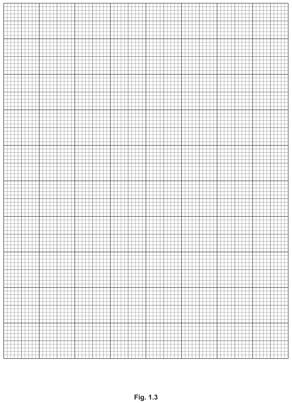
Fig. 1.3

3M Similar

DifficultyMedium

Worked solution

Answer

x-axis: percentage concentration of chloroplast suspension / % (linear scale 0–50 in steps of 10).
y-axis: rate of light-dependent stage of photosynthesis / $\text{s}^{-1}$ (linear scale 0–200 in steps of 50).
Points to plot: (10, 2.8); (20, 16.9); (30, 47.6); (40, 100.0); (50, 200.0) – each marked with a small, clear cross within $\pm \frac{1}{2}$ small square of its true position.
Line: a smooth curve drawn through (or as close as possible to) all five points – the data is non-linear, rising more steeply as concentration increases, so a straight line is not appropriate.

Final answer

Graph plotted with axes labelled, points accurate, smooth curve through the points.

Detailed explanation

Background Concept

A line graph is the correct choice for showing how a continuous variable (here, concentration) affects another continuous variable (here, rate). Each data point represents one observation, and the line (or curve) shows the underlying relationship. For data that follow a recognisable mathematical trend (here, an approximately exponential rise), a smooth curve of best fit is drawn rather than joining the points with a zig-zag.

Understanding the Question

You have five data points in Table 1.1 (after completing part (i)) and a blank grid in Fig. 1.3. You must draw a line graph: choose which variable goes on which axis, decide scales, plot the points, and draw an appropriate line.

Approach

Concentration is the independent variable (it is set by the experimenter) – put it on the x-axis. Rate is the dependent variable (it is measured) – put it on the y-axis. Choose scales that use at least half of the grid in each direction. Plot the points, then draw a smooth curve through them (the data is clearly non-linear – a straight line would distort the relationship).

Step-by-Step Reasoning

Axes orientation. Independent on the x-axis, dependent on the y-axis. Each axis labelled with the quantity and the unit in accepted form: 'percentage concentration of chloroplast suspension / %' and 'rate of light-dependent stage of photosynthesis / $\text{s}^{-1}$ '.
Scales. The largest rate is $200\ \text{s}^{-1}$ , so a y-scale of 0–200 in steps of 50 is appropriate and uses most of the grid vertically. The largest concentration is 50 %, so an x-scale of 0–50 in steps of 10 is appropriate and uses most of the grid horizontally. Avoid awkward scales (e.g. 0, 1, 2, 3, 4.7, 9.5 …) that make plotting difficult and waste grid space.
Plotting. Mark each point with a small × or • within half a small square of its true position.
Line. A smooth curve is best because the data rises more steeply at higher concentrations (a straight line of best fit would be a poor description of the relationship). The curve should pass through (or as close as possible to) every point and should not extend wildly beyond the data.

Key Takeaways

Independent variable on the x-axis, dependent on the y-axis.
Scales must use at least half the grid and be easy to read (multiples of 1, 2, 5 or 10).
A non-linear trend requires a smooth curve, not a straight line of best fit.
The plotted line should not be extrapolated beyond the range of the data without justification.

Common Mistakes

Swapping the axes (rate on x, concentration on y).
Forgetting the unit on the y-axis label, or writing 's' instead of ' $\text{s}^{-1}$ '.
Awkward scales (e.g. 0, 3, 7, 11, 15 …) that make plotting hard and waste grid space.
Joining the points with straight zig-zag segments instead of drawing a smooth curve.
Drawing the line all the way back to 0 % concentration (or far beyond 50 %) when the data do not support this.

Things to Be Careful About

The marks are split: one for axes, one for points, one for the line. Even if you draw a beautiful curve, you still need correct axes and accurate points to score all three.
Use a sharp pencil so the plotted points are clearly visible.

Techniques used

Plot a line graph on a gridChoose appropriate axis scalesDraw a suitable line through the points

(c)

The student initially trialled the experiment using ice-cold distilled water instead of ice-cold 10% sucrose to make the stock chloroplast suspension in step 1. The DCPIP did not decolourise.

Suggest why the procedure worked when 10% sucrose solution was used but did not work when distilled water was used in step 1.

2M Similar

DifficultyMedium

Worked solution

Answer

The 10% sucrose solution has (approximately) the same water potential as the stroma inside the chloroplasts (i.e. it is isotonic with the chloroplasts).
Therefore there is no (net) movement of water into the chloroplasts by osmosis (no water-potential gradient), so the chloroplasts do not burst / swell and the thylakoid membranes remain intact.
In distilled water the water potential outside the chloroplasts is much higher than inside, so water enters by osmosis, the chloroplasts swell and burst, destroying the thylakoid membranes; the light-dependent reactions cannot occur, the DCPIP is not reduced and so does not decolourise.

Final answer

10% sucrose is approximately isotonic with the chloroplast stroma, so no water enters by osmosis and the chloroplasts (and thylakoid membranes) remain intact; in distilled water the water-potential gradient causes water to enter by osmosis, the chloroplasts burst and the light-dependent stage cannot occur.

Detailed explanation

Background Concept

Osmosis is the net movement of water molecules across a partially permeable membrane down a water-potential gradient (from higher $\Psi$ to lower $\Psi$ ). Animal cells and organelles without a strong cell wall (such as chloroplasts) will swell and burst (lyse) if placed in a solution of much higher water potential (a hypotonic solution). The chloroplast's envelope and the thylakoid membrane system are not strong enough to resist a large osmotic influx. The 10% sucrose solution is conventionally used in chloroplast isolation because its water potential is close to that of the stroma inside an intact chloroplast, so chloroplasts remain intact and functional.

Understanding the Question

You are told that when the student used ice-cold distilled water instead of 10% sucrose to make the stock chloroplast suspension, the DCPIP did not decolourise. You need to explain why the 10% sucrose worked but the distilled water did not.

Approach

Identify what the 10% sucrose has that the distilled water lacks: a similar water potential to the chloroplast interior. Then trace the consequence: distilled water → steep water-potential gradient → osmotic water entry → chloroplasts burst → thylakoid membranes disrupted → no light-dependent reactions → DCPIP not reduced → no colour change.

Step-by-Step Reasoning

The 10% sucrose solution is approximately isotonic with the chloroplast stroma, so there is no (or only a very small) water-potential gradient across the chloroplast envelope.
With no gradient, no net osmotic movement of water occurs, so the chloroplasts retain their normal shape and the thylakoid membranes (the site of the light-dependent reactions) remain intact.
In distilled water the water potential outside the chloroplasts is much higher (closer to zero) than the stroma water potential, so water moves into the chloroplasts by osmosis.
The chloroplast envelope cannot withstand this osmotic influx; the chloroplasts swell and burst (lyse).
With the thylakoid membranes destroyed, the electron-transport chain can no longer operate, no electrons are available to reduce DCPIP, and the dye remains blue.

Key Takeaways

Isolated organelles must be kept in an isotonic solution to preserve membrane integrity.
Osmosis acts on organelles exactly as it does on whole cells.
10% sucrose is the standard osmotic buffer for chloroplast isolation in Cambridge practical work.

Common Mistakes

Saying the sucrose 'feeds' the chloroplasts or 'provides energy' – the role of the sucrose is purely osmotic, not nutritional.
Vague answers like 'the chloroplasts are damaged' – you must state why they are damaged (osmosis / bursting) and what is destroyed (the thylakoid membranes).
Confusing the direction of water movement (water moves from high $\Psi$ to low $\Psi$ , so it moves into the chloroplasts in distilled water).

Things to Be Careful About

The buffer at pH 7 (mentioned in step 1 of the procedure) protects the enzymes but does not protect against osmotic damage; the sucrose is the osmotic protector.
Both the ice-cold temperature and the sucrose are important: low temperature slows enzyme degradation, sucrose prevents osmotic bursting.

Techniques used

Explain the effect of water potential on chloroplastsApply knowledge of osmosis to organelle preservation

(d)

The preliminary experiment was carried out at $17^\circ\text{C}$ .

To investigate the effect of temperature on the rate of the light-dependent stage of photosynthesis, the student added some details to the instructions in steps 7, 8 and 9 to make sure that accurate results were recorded.

Describe an investigation that the student could follow to determine the effect of temperature on the rate of the light-dependent stage of photosynthesis.

• Use the results shown in Table 1.1 to decide on a suitable chloroplast suspension for the investigation.
• Include details of how you would take accurate results.
• Do not include a risk assessment.

Your method should be set out in a logical order and be detailed enough to allow another person to follow it.

6M Similar

DifficultyMedium-Hard

Worked solution

Answer

Choice of chloroplast suspension
Use 20% chloroplast suspension in 10% sucrose solution buffered at pH 7. (10% is too slow to be practical; 50% decolourises so quickly that the time cannot be measured accurately. 20% gives a measurable time of around 60 s and is a good compromise.)

Variables

Independent variable: temperature of the chloroplast suspension, e.g. 10, 20, 30, 40, 50, 60 °C (a minimum of five values across 10–60 °C).
Dependent variable: rate of the light-dependent stage $= 1000$ / time taken for the DCPIP to decolourise (in $\text{s}^{-1}$ ).
Standardised variables: volume of 20% chloroplast suspension (10 cm³); volume and concentration of DCPIP (1 cm³); same lamp at the same fixed distance from every tube; same pH; same concentration of sucrose.

Method

Prepare 20% chloroplast suspension in ice-cold 10% sucrose solution buffered at pH 7 as in steps 1–5 of the preliminary procedure.
Set a thermostatically controlled water bath to 10 °C and allow the temperature to stabilise.
Pipette 10 cm³ of the 20% chloroplast suspension into a flat-bottomed tube wrapped in black plastic film, add 1 cm³ of DCPIP solution and swirl gently to mix.
Place the tube in the 10 °C water bath for 5 minutes so that the suspension equilibrates to 10 °C.
Work in a dark room to prevent any stray light reaching the tube.
Position the bench lamp at a fixed distance (e.g. 10 cm) from the tube – the same lamp at the same distance for every trial.
Remove the black plastic film, start the stopwatch and record the time taken for the colour of the suspension to match a green colour standard (a reference tube containing chloroplast suspension alone, or a printed/tile green standard).
Calculate the rate using $\text{rate} = 1000/t$ .
Repeat steps 3–8 a further two times at 10 °C with fresh suspension to give three readings, and calculate the mean time (and mean rate) at 10 °C.
Repeat the entire procedure at 20, 30, 40, 50 and 60 °C, resetting the water-bath temperature each time, allowing it to equilibrate, and using fresh chloroplast suspension + DCPIP for each trial.
Plot a graph of rate (y-axis) against temperature (x-axis) to show the effect of temperature on the rate of the light-dependent stage.

Do not include a risk assessment (as instructed).

Final answer

Use 20% chloroplast suspension; test at least five temperatures between 10 and 60 °C; use a thermostatically controlled water bath and equilibrate the suspension to each temperature for 5 min before exposing it to the light; use the same lamp at the same distance; work in a dark room; judge the end-point against a green colour standard; repeat each temperature three times and calculate a mean.

Detailed explanation

Background Concept

Photosynthesis is catalysed by enzymes and by the membrane-bound photosystems in the thylakoid. Like all enzyme-catalysed processes, the light-dependent stage is temperature-dependent: as temperature rises, the kinetic energy of substrate and enzyme increases and the reaction rate rises (typically doubling for every 10 °C rise) up to an optimum (around 25–35 °C for most plant enzymes). Above the optimum the enzymes start to denature and the rate falls sharply. To investigate this effect, the rate must be measured at several temperatures while everything else is kept constant.

Understanding the Question

The student already has a procedure (the preliminary experiment) for measuring the rate of the light-dependent stage at one temperature (17 °C) using a chloroplast suspension + DCPIP. They now need to vary the temperature, measure the rate at each temperature accurately, and write a method detailed enough for another person to follow. Three practical challenges are central:

Choosing a chloroplast-suspension concentration that gives a measurable time (not too fast, not too slow).
Controlling and standardising the temperature during each measurement.
Judging the end-point (the moment all the DCPIP is reduced) accurately.

Approach

First, select a concentration from the preliminary data: 20% (or 30%) gives a measurable time without being impractically slow. Then identify the independent (temperature), dependent (rate) and standardised variables. Then describe the procedure in a logical order, addressing each practical challenge in turn. Finally, add the reliability step (repeats + mean).

Step-by-Step Reasoning

Choosing the concentration (mark-scheme point 1).
From Table 1.1:

10% → 351 s: too slow to be a practical rate measurement (almost 6 minutes per trial).
20% → 59 s: practical – about one minute per trial.
30% → 21 s: practical – about 20 s per trial.
40% → 10 s: getting too fast to time accurately with a stopwatch.
50% → 5 s: too fast to time accurately.

20% (or 30%) is the best compromise – a measurable time that still responds to changes in temperature. The mark scheme requires a stated concentration; any one of these is acceptable, but 20% is the cleanest choice.

Temperatures (mark-scheme point 2).
Use a minimum of five temperatures spanning 10–60 °C, e.g. 10, 20, 30, 40, 50, 60 °C. Five values let you see both the rising part of the curve and the falling part (enzyme denaturation) above the optimum. Stating the actual temperatures, rather than 'several', is what earns the mark.

Constant temperature (mark-scheme point 3).
The water bath must be thermostatically controlled so that the temperature of the suspension during exposure to light is the same as the temperature you set. A beaker of water at room temperature is not good enough – the lamp will warm it up over the course of the experiment.

Equilibration (mark-scheme point 4).
Place the tube in the water bath before exposing it to the lamp. If you take a tube at 10 °C and put it under a warm lamp, the suspension will heat up during the measurement, so the recorded rate is not the rate at 10 °C. 5 minutes is a typical equilibration time.

Swirling (mark-scheme point 5).
Swirl the tube just before exposing it to the lamp to ensure the temperature is uniform throughout the suspension (and to mix the DCPIP thoroughly with the chloroplasts).

Light intensity (mark-scheme point 6).
Use the same lamp, at the same distance, for every trial. The simplest way to standardise this is to mark the position of the lamp and the tube on the bench with tape.

Dark room (mark-scheme point 7).
Any stray light reaching the tube (other than from the lamp) will cause the light-dependent reactions to proceed and will affect the rate. Working in a dark room removes this uncontrolled variable.

End-point (mark-scheme point 8).
The end-point is the moment when all the DCPIP has been reduced and the suspension has the same green colour as chloroplast suspension alone. Because the eye is poor at judging a small colour change, a reference tube (or a printed green standard) is essential. A small amount of DCPIP is enough to colour the suspension blue-green; the moment the last trace of blue has gone, stop the clock.

Repeats and mean (mark-scheme point 9).
Repeat each temperature at least three times and calculate the mean time (and mean rate). The mean is the best estimate of the true rate; the spread of the repeats is a measure of experimental error.

Key Takeaways

A good plan must (i) identify the independent, dependent and standardised variables, (ii) state how each will be controlled, and (iii) describe the procedure in a logical, reproducible order.
Equilibration is essential: the variable you are varying must actually be at the value you think it is when you make the measurement.
Repeats and a mean are the minimum reliability step for a rate investigation.
An objective end-point (colour standard) is needed whenever the measurement is a colour change judged by eye.

Common Mistakes

Stating 'use a suitable concentration' without saying which one – the mark scheme specifically requires a stated concentration.
Vague temperature list ('20, 30, 40 °C') – you need at least five values, and they must span 10–60 °C.
Forgetting to equilibrate the suspension to the test temperature before exposing it to the lamp – this is a frequent omission and costs a mark.
Not standardising the lamp distance or working in ordinary room light – both introduce uncontrolled variation in light intensity.
Saying 'judge when the blue colour has gone' without specifying how the end-point is judged (colour standard / reference tube).
Describing the procedure without mentioning repeats and a mean.
Including a risk assessment – the question explicitly says do not include one.

Things to Be Careful About

The independent variable is the temperature of the suspension, not the temperature of the water bath. The two will not be exactly the same if you do not equilibrate.
Light intensity must be the same at every temperature; the lamp heats up over time, but its light output is what matters here.
Use a fresh tube of suspension + DCPIP for every trial, because the reaction consumes the DCPIP irreversibly.
A suitable graph for the result is rate (y-axis) against temperature (x-axis) – the rate rises to an optimum then falls sharply as the enzymes denature.

Techniques used

Plan an investigation to test the effect of temperatureStandardise light intensity and other variablesDetermine an end-point accuratelyRepeat experiments and calculate means

Q2Medium-HardPlanningAnalysis, Conclusions and Evaluation

The two-spot ladybird, Adalia bipunctata, is a species of small, flying beetle that is found in northern Europe and other parts of the world. The wings of these beetles are covered by two tough structures known as elytra, as shown in Fig. 2.1.

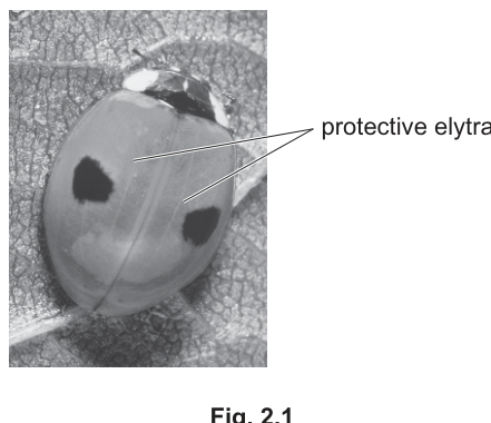
Fig. 2.1

A. bipunctata is an important predator of insect pests such as aphids. These insect pests feed on plants, including many crop species. Population numbers of A. bipunctata fluctuate in response to changes in the population numbers of their prey.

The elytra of A. bipunctata show phenotypic variation. The three most common morphs (forms) found in northern Europe are known as typica (T), quadrimaculata (Q) and sexpustulata (S).

• The typica morph, shown in Fig. 2.1, is mostly red with two black spots and is described as non-melanic.
• The other two morphs are described as melanic as they are mainly black with some red.
• The distribution of the colours in these three morphs is shown in Fig. 2.2.

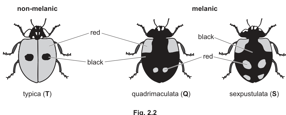
Fig. 2.2

In northern Europe, the populations of A. bipunctata hibernate (are inactive) during the winter. As the temperature increases in early spring, the populations become active. The populations remain active and produce three generations before the next winter begins.

(a)

It was observed that in some areas in populations of A. bipunctata, the proportion of non-melanic to melanic phenotypes in the early spring was different to the proportion later in the year in the autumn.

Researchers carried out a study in one area of Germany to compare the proportion of non-melanic to melanic phenotypes in early spring with the proportion in autumn after three generations had been produced. The data were collected over a period of 12 years.

The results are shown in Fig. 2.3.

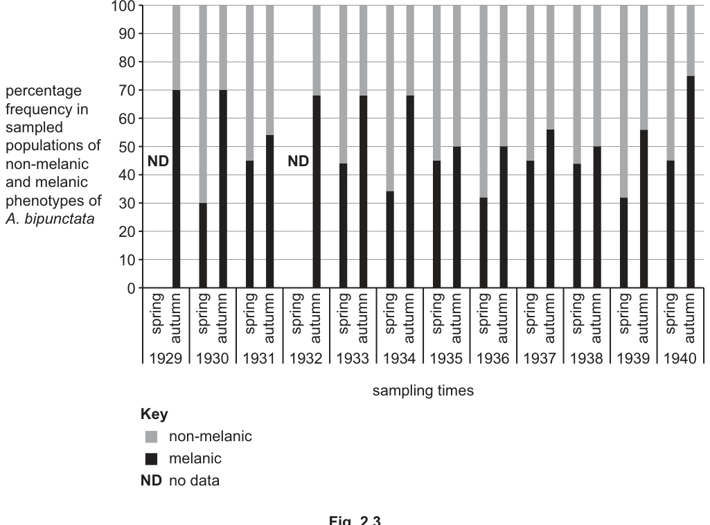
Fig. 2.3

(i)

Outline a method that could be followed to collect the data shown in Fig. 2.3.

3M Similar

DifficultyMedium-Easy

Worked solution

Answer

Use random or systematic sampling at the same sampling site(s) at the same time of year (early spring / autumn).
Collect the ladybirds using a suitable method such as quadrats, sweep nets, light traps or a pooter.
Count the number of each phenotype (non-melanic and melanic) collected in each sample so that the percentage frequency can be calculated for spring and autumn of each year.

Final answer

See answer

Detailed explanation

Background Concept

Fig. 2.3 is a stacked bar chart of percentage frequencies of non-melanic and melanic phenotypes in populations of Adalia bipunctata, sampled in spring and autumn over 12 years. To produce such data you must (i) take a representative sample of the population, (ii) count the individuals belonging to each phenotype and (iii) express the count of each as a percentage of the total. The reliability of the conclusion depends on sampling being unbiased (random or systematic), repeatable (same method each year) and on the sample being large enough.

Understanding the Question

The question asks the candidate to outline how the data shown in Fig. 2.3 could have been collected. The mark scheme expects three things: a description of the sampling strategy, identification of appropriate collecting equipment, and the act of counting/recording the phenotypes. A mark–release–recapture method is also acceptable but capped at 2 marks.

Approach

Choose the simplest practical sampling route that allows an estimate of phenotype frequency in the field. Ladybirds are small, flying beetles that occur on vegetation, so passive (quadrat) or active (sweep net / pooter) collection works; for flying insects a light trap is also valid. Emphasise that the same method, at the same sites, must be used in spring and in autumn so the comparison is fair.

Step-by-Step Reasoning

Sampling strategy — Use random sampling (e.g. randomly chosen coordinates within the area) or systematic sampling (e.g. transects / regularly spaced quadrats). Random/systematic sampling removes observer bias, which is the first marking point.
Apparatus — Collect the ladybirds using a method suited to small invertebrates on vegetation: quadrats, sweep nets, light traps or a pooter. This is the second marking point.
Counting — Within each sample, identify and count the number of non-melanic (typica, T) and melanic (Q and S) phenotypes. The numbers for each phenotype can then be converted into percentage frequencies, exactly as plotted in Fig. 2.3. This is the third marking point.

(Alternative, capped at 2: a mark–release–recapture scheme in which ladybirds are caught, counted by phenotype, marked harmlessly, then a second sample is taken and the recaptures counted by phenotype.)

Key Takeaways

Reliable ecological data on phenotype frequency depend on unbiased sampling and consistent methods across time points.
For small flying invertebrates, quadrats, sweep nets, light traps and pooters are all appropriate; mark–release–recapture can also estimate population composition.

Common Mistakes

Saying only "collect ladybirds" without naming a sampling strategy or an apparatus.
Describing mark–release–recapture fully but missing any one of: marking safely, releasing, recapturing, counting — which loses marks.
Confusing sweep netting (vegetation) with pitfall traps (ground-dwelling invertebrates).

Things to Be Careful About

The same sites/habitats must be sampled in spring and autumn each year; the data are only comparable if the protocol is standardised.
Marking must not harm the beetles, must not be quickly lost, and must not make them more conspicuous to predators than unmarked individuals.

Techniques used

describe a sampling protocol for an invertebrate populationselect appropriate collecting apparatusdescribe counting and recording phenotype frequencies

(ii)

The researchers concluded that there was a change in the proportion of the two phenotypes between spring and autumn, with the non-melanic phenotypes always showing a higher percentage frequency in the spring.

Suggest two pieces of extra information about the investigation that researchers should provide to improve confidence in their conclusion.

2M Similar

DifficultyMedium-Easy

Worked solution

Answer

Any two of:

The sample size (number of ladybirds collected) at each sampling time should be stated.
Sampling should be carried out at multiple sites within the same area of Germany (not just one site) to make the result representative.
A statistical test (e.g. chi-squared) should be applied to the spring vs autumn counts to test whether the difference is significant.
Data are missing for spring 1929 and spring 1932; these gaps should be filled or acknowledged.
Sampling should be standardised: same location(s)/habitat(s), same time of day and same duration of sampling in both spring and autumn.

Final answer

See answer

Detailed explanation

Background Concept

A conclusion about a real biological difference is only as strong as the evidence supporting it. Confidence in a comparison between two samples is increased by: (i) knowing how large each sample is, (ii) replicating the sampling across multiple sites and years, (iii) testing the difference statistically and (iv) standardising the protocol so the two samples are genuinely comparable.

Understanding the Question

The researchers concluded that the proportion of non-melanic to melanic phenotypes changes between spring and autumn (non-melanic higher in spring), based on Fig. 2.3. The question asks for two extra pieces of information that would improve confidence in that conclusion. Note that two spring bars (1929 and 1932) are labelled ND ("no data"), which is itself a confidence-limiting feature.

Approach

Look critically at what Fig. 2.3 does NOT show, and at the protocol that produced it. Candidates that score highest pick concrete, study-specific improvements rather than vague statements.

Step-by-Step Reasoning

Each of the following would improve confidence in the conclusion (any two from this list earn the two marks):

Sample size — the number of ladybirds counted in each spring/autumn sample is not given; without it the percentage frequencies are hard to compare meaningfully.
Multiple sampling sites within the same area of Germany would show whether the trend is local or general across the area.
Statistical analysis (e.g. a chi-squared test on the spring vs autumn counts each year, or a paired test across years) would tell us whether the observed differences are likely to have arisen by chance.
Missing data — spring 1929 and spring 1932 have no data ("ND"); filling or justifying these gaps would strengthen the 12-year trend.
Standardised protocol — same location(s)/habitat(s), same time of day and same duration of sampling in spring and autumn would ensure the comparison is fair.

Key Takeaways

A descriptive conclusion from a graph is strengthened by sample-size information, replication, statistical testing and a standardised protocol.
Always check whether data are missing or whether the comparison is fair; both reduce confidence if unaddressed.

Common Mistakes

Vague answers such as "do more trials" or "be more accurate" — these do not earn marks because they do not specify what to vary or measure.
Suggestions that go beyond the data (e.g. sequencing the gene) rather than addressing the reliability of the field study itself.

Things to Be Careful About

Improvements must be relevant to the study described; do not invent new hypotheses.
The mark scheme lists several acceptable suggestions; any two of them earn the two marks.

Techniques used

identify weaknesses in a study designsuggest improvements to strengthen a conclusion

(b)

Environmental temperature is one of many different selection pressures that could be acting on populations of A. bipunctata. The melanic phenotypes, morphs Q and S, are considered to be better adapted to the climate in northern Europe as they absorb heat energy more readily than the non-melanic phenotype, morph T.

Scientists investigated the effect of temperature on the body temperature of the two different phenotypes.

• The four individuals used in the investigation were collected while they were hibernating (inactive) and were kept outdoors for six weeks before the investigation.
• The individuals were weighed and arranged into pairs, each with approximately the same mass.
• A temperature sensor was fixed to the lower (ventral) surface of each individual.
• The temperature of each individual was recorded for 9 minutes. During that time, a heat-emitting lamp positioned directly above the individuals was switched on at 30s and switched off at 5 minutes.

The results are shown in Fig. 2.4.

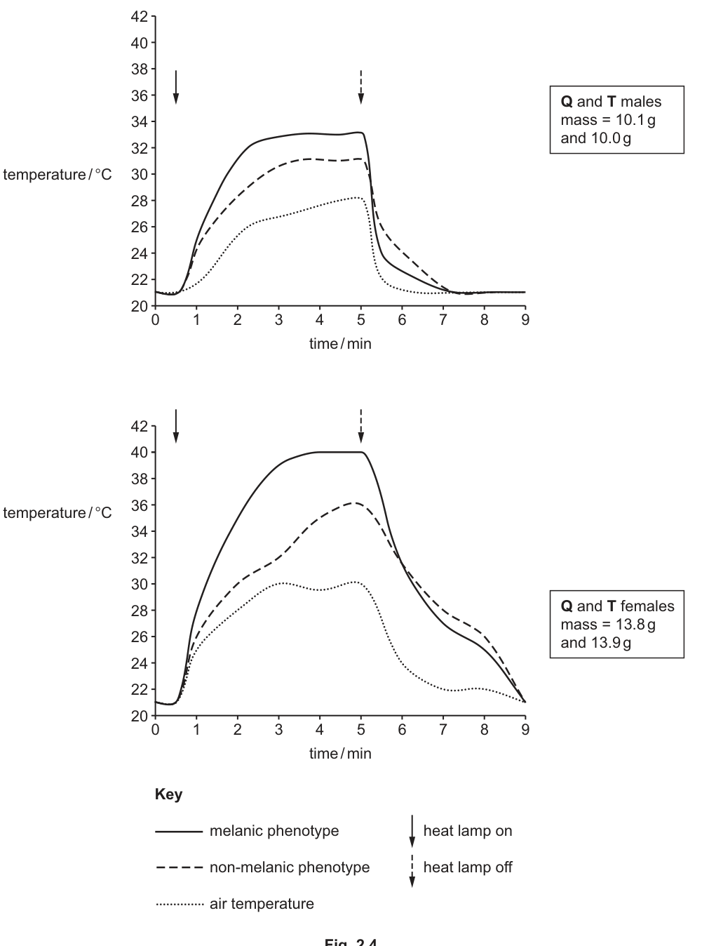
Fig. 2.4

(i)

The researchers concluded that melanic morphs warm up more quickly than non-melanic morphs.

Explain how the information shown in Fig. 2.4 supports this conclusion.

1M Similar

DifficultyMedium-Easy

Worked solution

Answer

In both graphs (males and females), the line for the melanic phenotype has a steeper gradient (rises more sharply) than the line for the non-melanic phenotype after the heat lamp is switched on, showing that the melanic morphs warm up more quickly.

Final answer

See answer

Detailed explanation

Background Concept

On a temperature-vs-time graph, the gradient (slope) of the line at any point represents the rate of temperature change (°C per minute). A steeper positive slope means the temperature is rising faster. The graph in Fig. 2.4 plots the body temperature of one melanic and one non-melanic ladybird under identical heat-lamp conditions, so differences in gradient can be attributed to the phenotype.

Understanding the Question

The researchers' conclusion is that "melanic morphs warm up more quickly than non-melanic morphs". The question asks how Fig. 2.4 supports this. The single mark is awarded for naming the observable feature that produces the conclusion — the gradient of the line.

Approach

Compare the slopes of the two lines (melanic vs non-melanic) during the period when the lamp is on. The steeper the slope, the faster the warming. This must be true in both the male graph and the female graph for the conclusion to be supported.

Step-by-Step Reasoning

In the top graph (males, ~10 g each), after the lamp is switched on at 0.5 min the melanic line rises more steeply than the non-melanic line, reaching a higher peak temperature.
In the bottom graph (females, ~13.8–13.9 g each), the same pattern is seen — the melanic line has a steeper gradient than the non-melanic line after the lamp is switched on.
Because a steeper gradient = faster rate of temperature increase, the steeper melanic line supports the conclusion that melanic morphs warm up more quickly than non-melanic morphs.

Key Takeaways

The gradient of a temperature-vs-time trace is the rate of temperature change.
A conclusion about "more quickly" must be backed up by a steeper gradient, not merely by a higher final value.

Common Mistakes

Saying "melanic reaches a higher temperature" — that addresses the peak, not the rate of warming.
Referring only to one of the two graphs when the conclusion is general.

Things to Be Careful About

"Steeper gradient" / "rises more sharply" is the precise language the mark scheme expects; vague phrases such as "the line goes up more" are too imprecise to earn the mark.

Techniques used

interpret a temperature-vs-time graphrelate the gradient of a line to the rate of warming

(ii)

State two further conclusions that can be made from the results shown in Fig. 2.4.

3M Similar

DifficultyMedium

Worked solution

Answer

Any two of the following (each must be supported by both graphs where applicable):

All four ladybirds start at the same body temperature (21 °C) before the lamp is switched on.
All four ladybirds warm up while the heat lamp is on and cool back down to the starting temperature after it is switched off.
Females (heavier, ~13.8–13.9 g) reach a higher peak temperature than males (~10.0–10.1 g) for both phenotypes.
Females (heavier) warm up more quickly (steeper gradient) than males (lighter).
The melanic morph cools down faster than the non-melanic morph after the lamp is switched off.

Final answer

See answer

Detailed explanation

Background Concept

Fig. 2.4 shows two temperature-vs-time traces, one for a pair of males (top) and one for a pair of females (bottom). In each pair, one individual is melanic and one non-melanic, and the sexes also differ in mass (males ~10 g, females ~13.8 g). The figure therefore separates the effects of phenotype and mass/sex on warming and cooling under a heat lamp. A "further conclusion" is one that goes beyond the conclusion already credited in b(i).

Understanding the Question

The question asks for two further conclusions that can be drawn from Fig. 2.4. The mark scheme explicitly requires that both graphs be used (one mark is reserved for that), and then two further substantive conclusions (each one mark) can be drawn from the list it provides.

Approach

Read both graphs carefully and look for features that are NOT the one credited in b(i) — i.e. features beyond "melanic warms faster than non-melanic". Candidate features include: shared starting conditions, behaviour when the lamp is off, sex/mass effects on warming rate and peak temperature, cooling rates, and plateauing.

Step-by-Step Reasoning

Possible further conclusions (any two earn the two further marks):

Common starting temperature — all four individuals begin at 21 °C, showing the protocol was properly standardised.
Common warming/cooling response — all four warm while the lamp is on and return to the starting temperature once the lamp is off, showing the response is reversible.
Sex/mass effect on peak — females (~13.8 g) reach higher peak temperatures than males (~10 g) for both phenotypes.
Sex/mass effect on rate — females (heavier) warm up more quickly (steeper slope) than males (lighter).
Sex/mass effect on cooling — females (heavier) take longer to cool down once the lamp is off.
Melanic cools faster — the melanic trace falls more steeply after the lamp is switched off than the non-melanic trace.
Plateau behaviour — the temperature plateaus for all individuals except the non-melanic females.

Key Takeaways

A multi-line graph lets you separate variables: in this case phenotype vs mass/sex.
"Further" conclusions must be additional to those already credited — describe features that go beyond warming rate by phenotype.

Common Mistakes

Restating the conclusion from b(i) — this earns nothing further.
Drawing a conclusion from only one of the two graphs when the comparison genuinely needs both.
Confusing "melanic cools faster" with "non-melanic stays warm longer" — these are equivalent but the mark scheme accepts either phrasing.

Things to Be Careful About

For full credit you must use both graphs (the first mark is reserved for this).
Each further conclusion should be a single, focused statement rather than several ideas run together.

Techniques used

extract additional conclusions from temperature-vs-time graphscompare male and female tracescompare light and heavy individuals

(c)

The scientists noticed that there appeared to be a relationship between body mass and the increase in body temperature. The scientists therefore continued to take results from another 17 individuals. They recorded the maximum difference between body temperature and the air temperature for each individual in their investigation.

All the results of the investigation are shown in Table 2.1 and Fig. 2.5.

Table 2.1

phenotype	morph	sex	mass/g	maximum temperature difference/ $^\circ\text{C}$
non-melanic	T	female	6.5	0.0
		male	8.4	1.1
		male	9.2	2.7
		male	10.0	2.9
		male	10.8	4.0
		female	11.5	5.4
		female	12.0	5.9
		female	13.1	5.3
		female	13.9	7.3
melanic	Q	male	8.4	3.5
		female	8.6	3.7
		male	10.1	5.3
		female	10.4	4.8
		female	11.0	8.5
		male	11.7	7.5
		female	13.1	7.3
		female	13.8	10.2
	S	male	8.6	4.1
		male	9.1	3.7
		male	10.8	5.9
		female	13.6	10.0

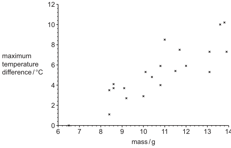
Fig. 2.5

State a statistical test that could be used to analyse the relationship shown in Table 2.1 and Fig. 2.5. Justify your choice.

statistical test ______

justification ______

3M Similar

DifficultyMedium

Worked solution

Answer

Statistical test: Pearson's (linear correlation)

Justification (any two):

The data for body mass and maximum temperature difference are paired (each individual contributes one value of each variable).
Both variables are continuous numerical data.
The scatter diagram (Fig. 2.5) shows the relationship is approximately linear (points lie around an upward-sloping straight line).
There are more than 5 paired observations (n = 21 individuals).

(Equally acceptable: Spearman's rank correlation, with justification that the data are paired and ordinal/interval, the scatter diagram shows an increasing relationship, and there are more than 5 observations.)

Final answer

Pearson's (linear correlation)

Detailed explanation

Background Concept

When you have two continuous, paired variables and you want to know whether they tend to vary together (and in which direction), the appropriate test is a correlation test. There are two common choices at A-level:

Pearson's linear correlation coefficient (r) — used when both variables are continuous and the scatter diagram suggests a linear (straight-line) relationship.
Spearman's rank correlation coefficient (rs) — used when the data are ordinal/interval or when the relationship is monotonic but not necessarily linear.

You are testing for an association, not a difference, so the t-test and chi-squared test are NOT appropriate here.

Understanding the Question

Table 2.1 gives the mass (g) and the maximum difference between body temperature and air temperature (°C) for 21 individual ladybirds, and Fig. 2.5 plots these as a scatter diagram showing a positive trend. The question asks for a statistical test that could analyse this relationship and a justification for the choice.

Approach

Decide what is being asked — is there a relationship between two continuous variables? → correlation, not difference.
Look at the scatter diagram — does it look linear or just increasing? → both Pearson's and Spearman's are defensible; Pearson's is the strongest choice because the relationship looks linear.
Tick off the assumptions of the chosen test: paired data, continuous variables, scatter suggests linear, n ≥ 5.

Step-by-Step Reasoning

Choosing the test

The question is about a relationship between mass and temperature difference, not about comparing two groups — so use a correlation test.
Both variables are continuous (mass in g, temperature difference in °C), and the scatter diagram shows an approximately linear upward trend, so Pearson's linear correlation is the most appropriate. Spearman's would also be accepted because the data are paired and there are clearly more than 5 observations.

Justification (any two from the following)

The data are paired — each individual contributes one mass and one temperature difference.
Both variables are continuous numerical data.
The scatter diagram (Fig. 2.5) shows the relationship is approximately linear (an upward-sloping straight line).
There are 21 paired observations, comfortably more than the minimum of 5.

Key Takeaways

A scatter diagram of two continuous variables → correlation, not t-test or chi-squared.
Justifying a test means naming the features of the data that meet the test's assumptions, not just stating the name.

Common Mistakes

Choosing the t-test (used for comparing two means) or chi-squared (used for counts/categories) — these are wrong here because there are no groups to compare.
Naming Pearson's but only giving justifications that apply to Spearman's (e.g. "ordinal data"), or vice versa.
Saying only "there is a relationship" without tying the justification to the actual scatter diagram.

Things to Be Careful About

Both Pearson's and Spearman's are acceptable; the mark scheme accepts either, but the justifications differ. Pick the test and match the justifications to that test.
The mark scheme's third justification is that the scatter diagram suggests a "linear relationship / correlation / association" — reference the figure explicitly.

Techniques used

choose an appropriate correlation testjustify the choice using features of the data and scatter diagram

(d)

The researchers assumed that the appearance of the elytra was controlled by a single gene with two alleles. Breeding experiments showed that the melanic phenotype is dominant to the non-melanic phenotype.

Researchers made the hypothesis:

Some melanics are homozygous dominant, and some melanics are heterozygous.

Outline a breeding experiment that could be carried out to test this hypothesis, and state the results you would expect if the hypothesis is supported.

3M Similar

DifficultyMedium-Hard

Worked solution

Answer

Cross each melanic ladybird with a non-melanic (homozygous recessive) partner.
Predicted results:
- Homozygous dominant melanic parent × non-melanic → all melanic offspring.
- Heterozygous melanic parent × non-melanic → a mixture of melanic and non-melanic offspring (approximately 1 : 1).
  Finding both types of outcome across the breeding pairs supports the hypothesis that some melanics are homozygous dominant and some are heterozygous.

Procedural details (any one):

Use many breeding pairs to give the result statistical reliability.
Keep each breeding pair separate from the others (or separate offspring from parents) so that each offspring can be assigned to the correct cross.
Count the phenotypes of the offspring in each cross and record the numbers.

Final answer

See answer

Detailed explanation

Background Concept

The elytral colour is controlled by a single gene with two alleles: melanic (M, dominant) and non-melanic (m, recessive). Phenotype alone cannot distinguish homozygous melanics (MM) from heterozygous melanics (Mm) because both look melanic. The standard genetic tool to reveal an unknown dominant-parental genotype is a test cross: cross the dominant-phenotype individual with a homozygous recessive (mm) partner. The offspring ratios distinguish the parental genotype:

\text{MM} \times \text{mm} \rightarrow \text{all Mm (all melanic)}

\text{Mm} \times \text{mm} \rightarrow \text{1 Mm : 1 mm (1 melanic : 1 non-melanic)}

Understanding the Question

The hypothesis is that some melanics are MM and some are Mm. The candidate must (i) design a breeding experiment that tests this and (ii) state the results expected if the hypothesis is supported. The mark scheme rewards naming the cross (melanic × non-melanic) and explicitly contrasting the two outcomes (all-melanic offspring vs mixed offspring) — plus one procedural detail.

Approach

A test cross is the natural design here, because the non-melanic phenotype tells us the genotype of that parent (mm) for certain. Use many independent crosses so that both parental-genotype classes have a chance to appear. Keep each cross separate so you can attribute each offspring to the correct parental pair, then count phenotypes.

Step-by-Step Reasoning

Set up the crosses — Pair each melanic ladybird (unknown genotype, MM or Mm) with a non-melanic partner (genotype mm, known from phenotype).
Separate and rear — Keep each breeding pair isolated from the others (e.g. in separate containers), so that each offspring can be assigned to its parents. Rear the offspring until the elytral phenotype is visible.
Record offspring phenotypes — Count the melanic and non-melanic offspring in each cross.
Interpret the results —
- A cross whose offspring are all melanic must come from a homozygous dominant (MM) melanic parent.
- A cross whose offspring are a mixture of melanic and non-melanic (approximately 1 : 1) must come from a heterozygous (Mm) melanic parent.
- Finding both kinds of cross outcome among many pairs supports the hypothesis that some melanics are MM and some are Mm.

Key Takeaways

When a phenotype can come from more than one genotype, a test cross to a homozygous recessive reveals the unknown parental genotype from the offspring ratios.
A controlled breeding experiment requires many pairs, isolation of each pair, and counting of offspring phenotypes.

Common Mistakes

Crossing two melanics together — this does not test the hypothesis because both parents could be MM, both Mm, or one of each, with several possible outcomes that cannot be unambiguously interpreted.
Crossing melanic × melanic and expecting all non-melanic offspring if the hypothesis is supported — wrong direction of cross.
Failing to keep the crosses separate, so offspring cannot be assigned to parents.
Saying "expect a 3 : 1 ratio" — that is the F2 of a monohybrid cross, not a test cross.

Things to Be Careful About

The mark scheme insists on BOTH predictions stated and contrasted: "homozygous dominant melanic parent → only melanic offspring AND heterozygous melanic parent → both phenotypes in offspring". A single outcome does not earn the second mark.
Use precise genetic terms: "homozygous dominant", "heterozygous", "homozygous recessive" (or equivalent genotype notation) — vague phrasing such as "pure-bred melanic" is acceptable but less rigorous.
One procedural detail (many pairs, isolation, or counting) earns the third mark; include at least one.

Techniques used

design a breeding experiment to test a genetic hypothesisapply the principle of a test crosspredict offspring phenotype ratios under dominant/recessive inheritance