Biology 9700/51 — October/November 2010
Cambridge A-Level · Planning, Analysis and Evaluation · worked solutions for every part, with the mark scheme
Topics Planning · Analysis, Conclusions and Evaluation
A student noticed that the leaves on a plant growing close to a wall had two sorts of leaves. The leaves next to the wall were in the shade and looked different from the leaves on the side away from the wall that were exposed to the sun. The length of the internodes on the stem also looked different.
The student decided to investigate the differences by measuring some features of 30 leaves and internodes from each side of the plant.
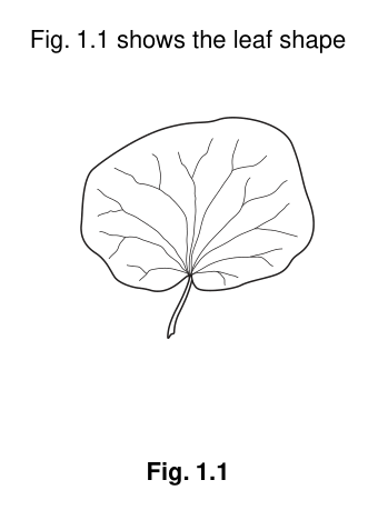
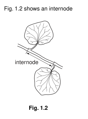
Table 1.1 shows the student’s results.
Table 1.1
| shaded leaves | exposed leaves | |
|---|---|---|
| mean internode length / | ||
| mean surface area of leaves / | ||
| mean mass of leaves / | ||
| mean leaf surface area : leaf mass ratio | ||
| rate of water loss / |
State the independent variable being investigated.
Answer
Light (intensity / exposure).
Light (intensity / exposure).
Background Concept
In any investigation, the independent variable (IV) is the factor the investigator deliberately varies (or selects) to study its effect on the dependent variable. Identifying the IV correctly is the first step in designing a sound experiment, because the IV determines what the two groups of samples are being compared on.
Understanding the Question
The student observed a single plant growing against a wall. One side of the plant faced the wall (shade) and the other side faced away (sun). The two sides had visibly different leaves and internodes. The student then measured the same set of features on leaves from each side. The question asks which variable the student is investigating — i.e. which factor differs between the two groups of leaves.
Approach
Compare the two sides of the plant: the only environmental factor that the student has allowed to differ is how much light each side receives. The student did not alter temperature, water supply, soil, or any other environmental factor. The IV must therefore be light.
Step-by-Step Reasoning
The two groups are: leaves on the shaded side of the plant, and leaves on the exposed (sunny) side of the plant. What differs between them is the light environment — specifically, the light intensity (or light exposure) reaching them. The mark scheme accepts "light intensity" or "light exposure" as the IV. It explicitly rejects: "light" on its own (too vague — could refer to wavelength, quality, etc.), and "position in shade/sun" (position is not what is being investigated; the underlying cause of the differences is the light).
Key Takeaways
- The IV is the factor the student varies (or selects) to study; here, it is the light reaching the two sides.
- Wording matters: the IV must describe the environmental factor, not the location.
Common Mistakes
- Writing "light" on its own — too vague.
- Writing "position", "location" or "side of plant" — these describe where, not what is being varied.
- Writing "sunlight" or "shade" — these are conditions, not the variable itself.
Things to Be Careful About
The mark scheme requires "light intensity" or "light exposure". Anything less specific (including "light" alone) is rejected.
Outline the procedures the student could use to obtain these results.
Answer
-
Systematic sampling of leaves — take every 3rd leaf from the apex on each side of the plant, or take leaves from the same height / position on the two sides, so that samples are comparable.
-
Surface area of each leaf — place the leaf on grid paper, draw around it, and count the full and part squares within the outline (or, for a round leaf, measure the diameter and use ). Add the two surfaces (upper and lower epidermis) together — or double one side — to get the total surface area.
-
Mass of each leaf — weigh each leaf on an electronic balance. For dry mass, dry the leaves in an oven at a low temperature until the mass is constant, then reweigh.
-
Internode length — measure with a ruler; alternatively, use string or cotton to mark the distance between two nodes and then measure the string against a ruler.
-
Water loss — set up a potometer and record the distance moved by the water meniscus (or air bubble) over a known time, OR weigh the leaf (or a sealed plastic bag enclosing it) at hourly intervals.
-
Control variables during water-loss measurement — keep temperature, humidity, air flow and light intensity constant for both sets of leaves while measuring transpiration.
-
Reliability — calculate the mean of all 30 leaves for each measurement; calculate the surface area : mass ratio for each leaf, then take the mean; calculate the standard deviation for each set of measurements.
-
Safety — this is a low-risk investigation; take care with hot equipment if an oven is used, and wash hands after handling leaves in case of any skin irritation.
See working: a systematic procedure covering sampling, surface area, mass (including dry mass), internode length, water loss with controlled conditions, reliability (mean, SD, SA:mass ratio) and safety.
Background Concept
A well-planned investigation requires clear identification of the independent variable, valid methods to measure the dependent variables, control of confounding variables, replication, calculation of summary statistics, and an honest assessment of safety. For an ecological or whole-organism study such as this, "valid" usually means a non-destructive, repeatable measurement on a representative sample, taken under standardised conditions.
Understanding the Question
Table 1.1 contains five measured features: mean internode length, mean leaf surface area, mean leaf mass, mean SA:mass ratio and mean rate of water loss. The candidate must outline a procedure that the student could have followed to obtain each of these values, plus cover reliability (mean, SD, ratio) and safety. The question is from Paper 5 (Planning, Analysis and Evaluation) so the answer should describe the procedure in enough detail to be replicated, but does not need to draw any apparatus.
Approach
Work through each measurement in turn, asking: (a) what is being measured, (b) which instrument or technique is appropriate, (c) how the result is calculated, (d) what conditions must be standardised. Then add a reliability section (mean, SD, SA:mass ratio) and a one-line safety section.
Step-by-Step Reasoning
Sampling. The student must obtain 30 leaves per side. To avoid bias, leaves should be sampled systematically — e.g. every 3rd leaf from the apex, or all leaves at a given height on each side. The mark scheme lists this as the first credit point.
Surface area. A flat leaf can be measured by tracing its outline on 1 mm² grid paper and counting full and part squares. For an approximately round leaf, measure the diameter and calculate area as . Because a leaf has two sides, the two surfaces must be added (or one side doubled) to give the total surface area — this is a separate credit point.
Mass. Weigh each leaf on an electronic balance, recording the value to a consistent precision (e.g. 0.01 g or 1 mg depending on the balance). The mark scheme additionally credits the idea of finding the dry mass: dry the leaves in an oven at a low temperature (e.g. 60–80 °C) until successive weighings give a constant mass. Dry mass removes variation caused by differing water content of the leaves.
Internode length. A simple ruler measurement is sufficient. For an intact plant, hold the ruler alongside the stem. For a cut section, lay the stem on the bench. An alternative is to wrap string around the internode, mark the length on the string, and then measure the string against a ruler — this is credited by the mark scheme as an alternative method.
Water loss. Two main methods are credited: a potometer, which records the distance moved by a water meniscus (or air bubble) in a capillary tube over a known time; or weighing the leaf (or a sealed bag enclosing the leaf) at hourly intervals and recording the decrease in mass. For both methods, the rate of water loss per unit area per unit time can be calculated. The conditions during the measurement (temperature, humidity, air movement, light) must be kept constant for both sets of leaves, or the comparison is invalid.
Reliability. Calculate the mean of all 30 leaves for each variable. Calculate the SA:mass ratio for each individual leaf (not the ratio of the means), then take the mean of those ratios. Calculate the standard deviation of each set of measurements so that the spread can be reported (as ± values in Table 1.1).
Safety. This is a low-risk investigation. If an oven is used for dry mass, take care with hot equipment. Wash hands after handling leaves in case of any skin irritation (the mark scheme notes "leaf allergy" as a possible issue).
Key Takeaways
- A sound procedure covers sampling, each measurement, control of variables, reliability and safety.
- For transpiration, the potometer or a weigh-and-go method both work; the environment must be standardised.
- The SA:mass ratio must be calculated per leaf (then averaged), not from the two means.
- Dry mass removes the confounding effect of variable water content.
Common Mistakes
- Picking leaves by eye (biased) instead of sampling systematically.
- Reporting a single leaf's data rather than the mean of 30.
- Using fresh mass only and ignoring dry mass.
- Calculating SA:mass as (mean SA) ÷ (mean mass) instead of as the mean of the individual ratios.
- Forgetting to standardise temperature, humidity, air flow and light during water-loss measurement.
- Not including standard deviation in the reliability section.
Things to Be Careful About
- 8 marks are available from 14 possible marking points. The dependent-variables section is capped at 6 of 9 points, even if you cover all of them.
- "Both sides" of a leaf means upper + lower surface, not the two sides of the plant.
- Do not mention planting seeds or potted plants — the mark scheme explicitly ignores this.
The student carried out -tests for leaf surface area : leaf mass ratio and for internode length.
The leaf surface area : leaf mass ratio gave the value
The formula for -test is
Complete the calculation to find the value of for the internode length.
Show your working.
= ______
Working
Answer
(allow 8.89 / 9)
8.9
Background Concept
The two-sample t-test compares the means of two independent groups and produces a single statistic, , that measures how many standard errors apart the two means are. The formula is
where is the mean, is the standard deviation and is the sample size. The larger is, the more confidently the two groups can be considered genuinely different.
Understanding the Question
The question gives the means (23 and 15), the standard deviations (4 and 3) and the sample sizes (30 and 30) for internode length, and asks the candidate to fill in the blanks in the t-test equation and calculate the value of . The answer must include the working.
Approach
- Take the difference of the means (numerator): .
- Substitute the standard deviations and sample sizes into the denominator and simplify: , so (rounded to 1 s.f. as in the question).
- Divide: , reported as (2 s.f.).
Step-by-Step Reasoning
The shaded internodes have mm and mm; the exposed internodes have mm and mm; both samples have .
- Numerator: .
- Denominator first term: .
- Denominator second term: .
- Sum: .
- Square root: , which the question rounds to 0.9.
- Final ratio: , which rounds to 8.9.
Key Takeaways
- A t-test summarises "how far apart are two means, in units of standard error?".
- The result of a t-test is then compared to a critical value at the appropriate degrees of freedom to test for statistical significance.
Common Mistakes
- Forgetting the absolute value (t should be positive).
- Using instead of in the denominator.
- Using the wrong n (n is per sample, 30 — not the combined 60).
- Reporting from the unrounded denominator 0.9129 (the question stipulates 0.9, so 8.9 is the expected answer).
Things to Be Careful About
- The mark scheme accepts 8.9, 8.89, 9 and 8.88... (the more precise value).
- Error carried forward (ecf) is allowed if the numerator is wrong.
Table 1.2 shows the critical values at for the -test.
Table 1.2
| degrees of freedom | 18 | 20 | 21 | 22 | 23 | 24 | 25 | 26 | 27 | 28 | 29 | 30 | 40 | 60 | |
|---|---|---|---|---|---|---|---|---|---|---|---|---|---|---|---|
| critical value | 2.10 | 2.09 | 2.08 | 2.07 | 2.06 | 2.06 | 2.06 | 2.06 | 2.05 | 2.05 | 2.04 | 2.04 | 2.02 | 2.00 | 1.96 |
The number of degrees of freedom is 58.
State how the number of degrees of freedom was calculated.
Answer
Degrees of freedom =
(Equivalently, .)
, or equivalently .
Background Concept
For a two-sample t-test, the degrees of freedom (df) represent the number of independent values that can vary once the two sample means are fixed. Each sample contributes df because the mean "uses up" one degree of freedom, so the total is , or simply .
Understanding the Question
The student used 30 leaves per group, so . The question tells the candidate that df = 58 and asks how this number was obtained. The expected answer is the formula or the explicit sum.
Approach
Apply the formula df = . Substitute .
Step-by-Step Reasoning
.
Equivalently, .
Key Takeaways
- For a two-sample t-test, df = .
- df is needed to look up the critical value in a t-table.
Common Mistakes
- Writing (forgetting to subtract 2).
- Writing (this is not the formula).
- Confusing with df for a chi-squared test (= number of categories − 1).
Things to Be Careful About
The mark scheme accepts any equivalent expression, including or .
State and explain the meaning of these results.
Answer
At 58 degrees of freedom, the critical value at is . Both calculated values (12.6 for the SA:mass ratio and 8.9 for internode length) are greater than .
Both differences between shaded and exposed leaves are therefore statistically significant (unlikely to be due to chance) and are likely to be caused by the difference in light exposure between the two sides of the plant.
Both calculated t-values (12.6 and 8.9) are greater than the critical value of 2.00 at df = 58, so both differences are statistically significant and likely to be caused by the difference in light exposure.
Background Concept
A t-test result is interpreted by comparing the calculated to a critical value at the chosen significance level (usually ) and the relevant degrees of freedom. If critical value, the difference between the two means is statistically significant — i.e. the null hypothesis (that the two samples come from populations with the same mean) can be rejected. If critical value, the difference is not significant and the null hypothesis stands.
Understanding the Question
Two t-values are available: for the SA:mass ratio and (from part (b)(i)) for internode length. With df = 58, the critical value at is 2.00 (the mark scheme rounds df = 58 to 60, whose critical value is 2.00). The question asks the candidate to state and explain what these results mean biologically.
Approach
- Read the critical value at df = 58 (effectively 60) and from Table 1.2: it is 2.00.
- Compare both calculated t-values to 2.00.
- State the conclusion and link it back to the independent variable (light exposure).
Step-by-Step Reasoning
- for SA:mass ratio > 2.00 → the difference in SA:mass ratio between shaded and exposed leaves is statistically significant.
- for internode length > 2.00 → the difference in internode length is also statistically significant.
- Because both p-values are below 0.05, we reject the null hypothesis for both features. The differences are very unlikely to be due to chance and are most plausibly caused by the difference in light exposure between the two sides of the plant.
Key Takeaways
- critical value → statistically significant → reject the null hypothesis.
- A larger means stronger evidence of a real difference.
- The conclusion should link the significant difference to the independent variable.
Common Mistakes
- Saying "the difference is not significant because 8.9 < 12.6" (8.9 is still > 2.00, so it IS significant).
- Stating "we accept the null hypothesis" when critical value (it should be "we fail to reject the null hypothesis").
- Not mentioning the critical value at all.
Things to Be Careful About
- The mark scheme allows ecf from (b)(i).
- The mark scheme ignores any mention of "null hypothesis" unless explained in context.
In a further investigation, the student cut sections of the leaves from the shaded side and from the exposed side of the plant. The following procedures were carried out:
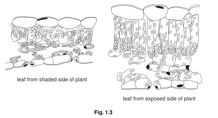
Transverse sections were made of each leaf and high-power drawings were made from these sections. The relative thickness of both the leaf and the cuticle were measured using an eyepiece graticule and the difference in the distribution of chloroplasts was observed.
Fig. 1.3 shows drawings made from transverse sections of these leaves.
Explain how the actual thickness of the leaf could be measured.
Answer
-
Calibrate the eyepiece graticule — place a stage micrometer on the stage, focus the microscope, and align the graticule and stage-micrometer scales. Determine how many graticule units equal a known length on the stage micrometer, and so find the actual length represented by one graticule unit at that magnification.
-
Measure the leaf section — replace the stage micrometer with the leaf transverse section, count the number of eyepiece graticule units across the leaf, and convert the count to an actual length by multiplying by the value of one graticule unit.
Calibrate the eyepiece graticule using a stage micrometer to find the actual length of one graticule unit; then count the number of graticule units across the leaf and convert to an actual length.
Background Concept
An eyepiece graticule is a small glass disc, marked with a linear scale, that sits in the eyepiece of a microscope. Because the size of the image depends on the objective lens in use, the graticule's units are arbitrary until they are calibrated. The calibration is done using a stage micrometer, a slide with a precisely known scale (typically 1 mm divided into 100 parts of 0.01 mm, or 2 mm divided into 200 parts).
Understanding the Question
The student has cut transverse sections of the leaves and needs to find the actual (i.e. real, in mm or µm) thickness of the leaf, not the apparent thickness in graticule units. The question asks how this is done.
Approach
A two-step method: (1) calibrate the graticule for the objective lens being used, (2) apply the calibration to the specimen.
Step-by-Step Reasoning
Step 1: calibration.
- Place the stage micrometer on the microscope stage and bring its scale into focus using the same objective lens that will be used for the specimen.
- Rotate the eyepiece (or slide the micrometer) until the graticule scale and the stage-micrometer scale lie alongside each other.
- Identify two points where the two scales coincide, count how many graticule units and how many stage-micrometer divisions lie between those points, and calculate the actual length of one graticule unit. For example, if 50 graticule units align with 0.5 mm on the stage micrometer, then 1 graticule unit = 0.5 / 50 mm = 0.01 mm = 10 µm.
Step 2: measurement.
- Replace the stage micrometer with the leaf transverse section.
- Count the number of graticule units across the leaf (i.e. between the upper and lower epidermis, perpendicular to the surface).
- Multiply by the calibration value: actual thickness = (number of graticule units) × (value of one unit).
Note. The calibration must be repeated for each objective lens, because the apparent size of one graticule unit changes with magnification.
Key Takeaways
- An eyepiece graticule measures in arbitrary units; it must be calibrated for the objective lens in use.
- The stage micrometer is the standard against which the graticule is calibrated.
Common Mistakes
- Counting graticule units and reporting that as the answer (the units must be converted to an actual length).
- Failing to specify that the calibration is done at the same objective lens as the measurement.
- Using a ruler on the projected image (acceptable for a low-power plan, but the question is about a microscope section).
Things to Be Careful About
- The mark scheme requires both: (a) counting the graticule units across the leaf, and (b) calibrating the graticule with a stage micrometer. One point each.
With reference to the student’s results, state what conclusions can be drawn about the differences in adaptations shown by shaded leaves and exposed leaves of the plant.
Answer
Shade leaves — adaptations to maximise light capture in low light
- Their larger surface area ( vs ) gives a bigger area to absorb the limited light available.
- The higher SA:mass ratio ( vs ) reflects a thinner leaf (confirmed by the single palisade layer and loosely packed spongy mesophyll in Fig 1.3), so light can penetrate to all the chloroplasts.
- A thinner cuticle is a smaller barrier to light penetration, so more light reaches the photosynthetic cells.
- The loosely packed spongy mesophyll with larger air spaces (visible in Fig 1.3) allows better gas diffusion for photosynthesis.
Exposed leaves — adaptations to limit water loss in high light
- A thicker cuticle reduces water loss by evaporation.
- The smaller surface area () reduces the total area from which water can be lost.
- The densely packed spongy mesophyll with smaller air spaces (visible in Fig 1.3) reduces water loss.
- The two layers of palisade mesophyll contain more chloroplasts and so can absorb the abundant light available.
Shade leaves are adapted to maximise light capture (larger surface area, higher SA:mass ratio = thinner leaf, thinner cuticle, single palisade layer, loosely packed spongy mesophyll); exposed leaves are adapted to limit water loss (thicker cuticle, smaller surface area, denser spongy mesophyll) while still maximising light capture (two palisade layers packed with chloroplasts).
Background Concept
Plants show phenotypic plasticity in their leaves in response to light environment. Shade leaves are typically larger, thinner, with a single palisade layer and a thinner cuticle — features that maximise the capture of the limited light available. Sun (exposed) leaves are typically smaller, thicker, with multiple palisade layers and a thicker cuticle — features that both capture abundant light AND reduce water loss, which is high in sunny, dry conditions. This is a classic trade-off: in shade, light is limiting; in sun, water is limiting.
Understanding the Question
The candidate is given two sources of information:
- Table 1.1 — quantitative measurements (surface area, mass, SA:mass ratio, water-loss rate) on 30 leaves from each side.
- Fig 1.3 — high-power drawings of transverse sections of leaves from each side, showing the cuticle, palisade and spongy mesophyll.
The question asks the candidate to draw conclusions about the adaptations of the two leaf types, referring back to the student's results. The mark scheme explicitly states that the answer should not simply restate the data; it must give a conclusion about adaptation. Any reference to growth, internodes or stomata is ignored.
Approach
For each leaf type:
- Note the key features in Table 1.1 and Fig 1.3.
- Link each feature to a biological advantage (light capture for shade leaves; water conservation for sun leaves).
- State the overall conclusion for that leaf type.
Step-by-Step Reasoning
Shade leaves (from Table 1.1 and Fig 1.3).
- Mean surface area = (vs for exposed) → a larger area to capture limited light.
- Mean SA:mass ratio = (vs for exposed) → a much thinner leaf per unit area, so light does not have to travel through much non-photosynthetic material.
- The transverse section (Fig 1.3) shows a single layer of palisade mesophyll cells, a loosely packed spongy mesophyll with large air spaces, and (implied) a thinner cuticle.
- These features are all consistent with maximising light capture: a thin leaf lets light through, a single palisade layer is enough because the light is not intense, the loose spongy mesophyll allows efficient gas diffusion, and a thin cuticle is a small barrier to incoming light.
Exposed leaves (from Table 1.1 and Fig 1.3).
- Mean surface area = (vs for shaded) → smaller area, less water lost by evaporation.
- Mean SA:mass ratio = (vs for shaded) → a thicker, heavier leaf per unit area.
- The transverse section (Fig 1.3) shows a much thicker cuticle, two layers of palisade mesophyll cells packed with chloroplasts, and a more densely packed spongy mesophyll with smaller air spaces.
- These features are all consistent with minimising water loss (thicker cuticle, denser packing, smaller surface area) while still maximising light capture (two palisade layers = many chloroplasts close to the upper surface, able to absorb the abundant light).
Overall. The data and the structural observations together show that shade leaves are adapted to maximise photosynthesis in low light, while sun leaves are adapted to limit water loss in high light (and still photosynthesise efficiently thanks to extra palisade tissue).
Key Takeaways
- Shade leaves → maximise light capture.
- Sun leaves → minimise water loss (and still capture light with extra palisade tissue).
- The SA:mass ratio is a useful proxy for leaf thickness.
- Multiple lines of evidence (measurements + structure) should be combined into a single coherent argument.
Common Mistakes
- Restating the data without giving a conclusion about adaptation (the mark scheme explicitly does not credit this).
- Including the rate of water loss as a "limitation" of the data (it is a result, not a limitation).
- Mentioning internodes, stomata or growth (the mark scheme ignores all of these).
- Mixing up the leaf types — saying e.g. "shade leaves have a thicker cuticle" reverses the correct conclusion.
Things to Be Careful About
- The mark scheme gives 5 possible points for shade leaves and 5 for sun leaves, and accepts a mix-and-match as long as the candidate is clear about which leaf type each point refers to. Take care not to give the same biological idea twice (e.g. "thinner leaf" and "single palisade layer" are different points; "thicker cuticle" and "denser packing" are different points).
The rest of this paper
1 more questions- Q2Planning · Analysis, Conclusions and Evaluation10M