Physics 5054/42 — October/November 2017

Cambridge O-Level · Alternative to Practical · worked solutions for every part, with the mark scheme

questions

marks

minutes

Topics Experimental Contexts · Observations and Measurements · Analysis, Conclusions and Evaluation · Use of Techniques, Apparatus and Materials · Planning Experiments and Investigations

Q1Experimental ContextsObservations and MeasurementsAnalysis, Conclusions and EvaluationUse of Techniques, Apparatus and MaterialsFree sample

A student investigates the period of a simple pendulum. The period $T$ is the time taken for one complete oscillation of the pendulum.

She sets up the pendulum with its point of support a fixed height above the surface of the bench. She does not change this height, or the position of the clamp during the investigation.

A scale diagram of her experimental set-up is shown in Fig. 1.1.

Fig. 1.1

(a)

(i)

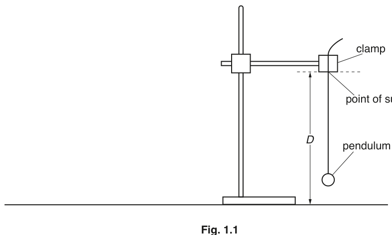
Measure the distance $D$ on Fig. 1.1 to the nearest millimetre. Record your result.

$D$ = ______ $\text{cm}$

(ii)

Fig. 1.1 is drawn to a scale of one-tenth full size.

Write down the actual height $H$ of the point of support above the bench.

$H$ = ______

(b)

She adjusts the length of the thread until the height $h$ of the centre of the bob above the bench is 15.0 cm. She gives the ball a small sideways displacement and releases it so that it oscillates. She records the time for 20 oscillations in the table in Fig. 1.2.

Fig. 1.2

$h / \text{cm}$	time for 20 oscillations / $\text{s}$	$T / \text{s}$	$T^2 / \text{s}^2$
15.0	22.8
20.0	20.8	1.04	1.08
25.0	18.8	0.94	0.88
30.0	16.6	0.83	0.69
40.0	10.6	0.53	0.28

She repeats the procedure for heights $h$ of 20.0 cm, 25.0 cm, 30.0 cm and 40.0 cm.

She uses her results to calculate the period $T$ for one oscillation and $T^2$ for each set of readings.

(i)

Complete the table in Fig. 1.2.

(ii)

Explain why measuring the time for 20 oscillations, rather than for 1 oscillation, gives a more accurate value for $T$ .

(c)

(i)

On Fig. 1.3, plot a graph of $T^2 / \text{s}^2$ on the $y$ -axis against $h / \text{cm}$ on the $x$ -axis.

Start your axes from the origin (0,0). Draw the straight line of best fit.

Fig. 1.3

(ii)

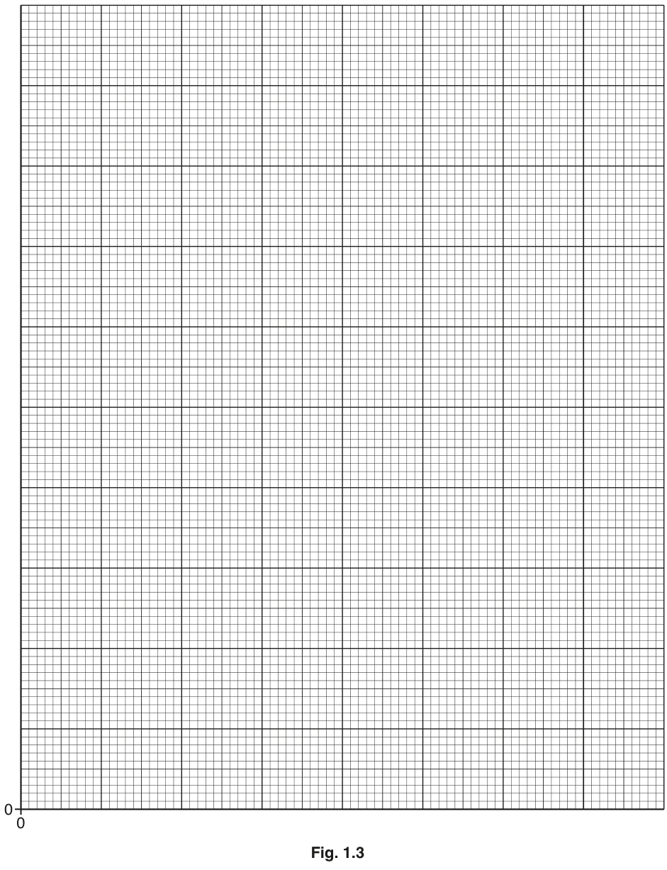
Extend your line so that it cuts the $y$ -axis.

State the value of the intercept $c$ on the $y$ -axis.

$c$ = ______ $\text{s}^2$

(iii)

Calculate the gradient $m$ of your line. Show your working and indicate on your graph the values you use to calculate the gradient.

$m$ = ______ $\text{s}^2 / \text{cm}$

(d)

Theory suggests that $H$ is given by the equation

H = \frac{c}{m}

Use this equation to calculate $H$ .

$H$ = ______ $\text{cm}$

(e)

Compare your measured value for $H$ from (a)(ii) with your result in (d).

State whether the two values agree with each other and justify your answer.

The rest of this paper

3 more questions

Q2Observations and Measurements · Experimental Contexts · Analysis, Conclusions and Evaluation · Use of Techniques, Apparatus and Materials · Planning Experiments and Investigations7M
Q3Experimental Contexts5M
Q4Use of Techniques, Apparatus and Materials · Experimental Contexts · Planning Experiments and Investigations · Observations and Measurements · Analysis, Conclusions and Evaluation5M

Loading the full paper…