Physics 5054/42 — October/November 2012
Cambridge O-Level · Alternative to Practical · worked solutions for every part, with the mark scheme
Topics Observations and Measurements · Experimental Contexts · Use of Techniques, Apparatus and Materials · Analysis, Conclusions and Evaluation · Planning Experiments and Investigations
A student investigates the speed of water waves.
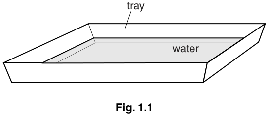
A rectangular plastic tray has a layer of water in the bottom, as shown in Fig. 1.1.
One end of the tray is lifted gently a small distance, as shown in Fig. 1.2a. When the water is still, the tray is lowered quickly. This causes a wave to travel across the surface of the water, as shown in Fig. 1.2b.
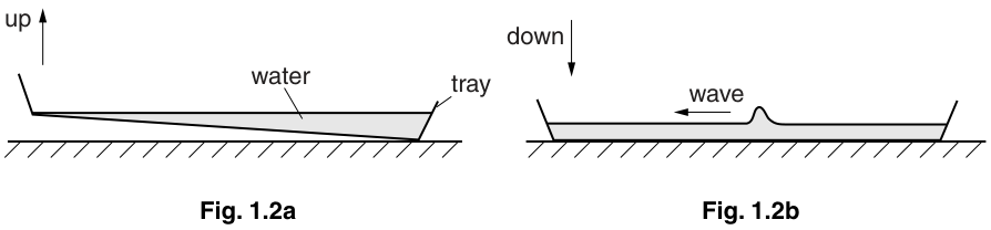
The wave is reflected by the ends of the tray and travels backwards and forwards several times.
The student estimates the time for the wave to travel one length of the tray to be about one second.
Suggest a reason why the student decides to measure the time for the wave to travel five lengths of the tray.
Answer
The time for one length is very short (about ), so human reaction time would cause a large percentage error. Measuring five lengths increases the total time and gives a more accurate average time.
Measuring five lengths reduces the percentage error due to reaction time and gives an average time
Walkthrough
When measuring short time intervals (around ), human reaction time (typically to ) contributes a very large fraction of the total measurement (up to ).
By measuring the time taken for the wave to travel 5 lengths of the tray, the total measured time becomes about . The reaction time remains roughly the same absolute value (about ), so its percentage impact drops to around . Dividing this total time by 5 gives a much more accurate average value for the time of one length.
Key Takeaways
- For very short events, timing multiple oscillations, cycles, or passes significantly reduces the relative (percentage) error caused by human reaction time.
- It also averages out minor variations in individual wave passes.
Common Mistakes
- Stating simply "to be more accurate" without explaining that it reduces the effect of human reaction time or provides an average.
- Claiming it eliminates human error entirely; it only reduces the percentage uncertainty.
Things to Be Careful About
- Always link the reason to the specific context given in the question: the time for one length is small ().
The ends of the tray slope outwards.
Explain why this makes it difficult to measure accurately the distance travelled by the wave.
Answer
The length of the tray varies from the bottom to the top because the sides slope outwards, making it difficult to place a ruler directly adjacent to the water surface.
The distance travelled / length of the tray varies with height and the ruler cannot be placed close to the water
Walkthrough
Because the ends of the tray slope outwards, the internal length of the tray is shorter at the base than at the top rim. As the depth of water changes, the exact distance the wave travels between the two reflecting walls also changes slightly. Furthermore, a standard straight ruler cannot sit flush against the water surface right up against the sloping wall, making precise alignment challenging.
Key Takeaways
- Irregular or non-vertical geometry introduces uncertainty in defining where a path starts and ends.
- Sloping walls mean distance depends on the height (depth) at which it is measured.
Common Mistakes
- Giving vague answers like "the ruler is too short" or "the water moves".
Things to Be Careful About
- Focus directly on the effect of the sloping ends as stated in the question.
Describe a possible method of measuring the distance travelled by the wave.
You may use a diagram in your answer.
Answer
Place a ruler horizontally across the top of the tray and view vertically from above (perpendicularly) to read the positions of the water boundaries, or use a flexible measuring tape along the water level.
View a ruler from vertically above the water surface (or use a flexible tape measure at the water surface)
Walkthrough
To overcome the difficulty caused by the sloping ends:
- Method 1 (Ruler with vertical alignment): Place a rigid ruler above the tray horizontally and sight vertically downwards (at right angles to the ruler) to avoid parallax error when aligning the ends of the water surface with the scale.
- Method 2 (Set squares): Use set squares placed vertically against the ends at the water level to project the position up to a horizontal ruler.
- Method 3 (Flexible tape): Use a flexible measuring tape placed directly along the surface of the water between the reflecting ends.
Key Takeaways
- Viewing a ruler perpendicularly prevents parallax error when the ruler cannot touch the object directly.
- Auxiliary tools like set squares or flexible tapes help transfer measurements accurately from awkward geometries.
Common Mistakes
- Not specifying the viewing angle ("look at it") which loses the technique mark.
Things to Be Careful About
- Clearly state how the measurement is taken accurately (e.g., viewing vertically from above).
The student measures the depth of the water. He has two identical rulers.
Part of one ruler is shown in Fig. 1.3.
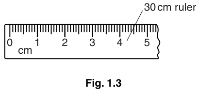
Explain why it is difficult to measure using only one of these rulers.
Answer
There is an ungraduated dead space (gap) between the physical end of the ruler and the mark, so the zero mark does not touch the bottom of the tray when the ruler is placed vertically in the water.
There is a dead space / gap before the zero mark, so the zero mark does not reach the bottom of the tray
Walkthrough
Looking at Fig. 1.3, the zero graduation line is not located exactly at the physical edge of the plastic ruler; there is a blank gap (dead space) of several millimetres. If the ruler is stood vertically in the tray with its end resting on the bottom, the water level will be read against the scale, but the measurement will omit the height of this ungraduated gap, leading to an incorrect (underestimated) reading for the depth .
Key Takeaways
- Most standard laboratory rulers have blank plastic margins before the mark, which acts as a zero offset when measuring depth directly.
Common Mistakes
- Confusing the dead space with parallax error.
- Simply stating "the ruler starts at zero" without mentioning the physical end of the ruler extends beyond zero.
Things to Be Careful About
- Be precise: refer to the space/gap between the physical end of the ruler and the line.
Describe a method of measuring using the two rulers.
You may use a diagram in your answer.
Answer
- Use the second ruler to measure the length of the dead space (the distance from the physical end of the first ruler to its mark).
- Place the first ruler vertically into the water with its end on the bottom of the tray, read the water level on the scale, and add the measured dead space to this reading to find .
Measure the dead space using the second ruler, then add this length to the depth reading from the first ruler
Walkthrough
To obtain the true depth using two rulers:
- Measure the offset: Use the graduated scale of Ruler 2 to measure the exact length of the ungraduated end margin (dead space) on Ruler 1.
- Measure the water level: Stand Ruler 1 vertically on the bottom of the tray and note the reading where the water surface meets the scale.
- Calculate total depth: The true depth is:
Alternatively, Ruler 2 can be placed horizontally across the top of the tray and Ruler 1 inverted/lowered, but measuring and adding the end offset is the standard, robust method credited by the mark scheme.
Key Takeaways
- When an instrument has a fixed zero offset, measuring the offset with another instrument and adding/subtracting it yields the correct value.
Common Mistakes
- Forgetting to explicitly state that the measured dead space must be added to the reading on the ruler.
Things to Be Careful About
- Ensure both marking points are met: (1) measure the dead space with the second ruler, (2) add this dead space to the reading.
The student repeats the experiment for different values of and calculates the speed of the wave for each value of .
Fig. 1.4 shows the student's results.
Fig. 1.4
| 0.5 | 20.6 |
| 1.0 | 28.5 |
| 1.5 | 35.5 |
| 2.0 | 42.0 |
| 2.5 | 46.3 |
| 3.0 | 50.5 |
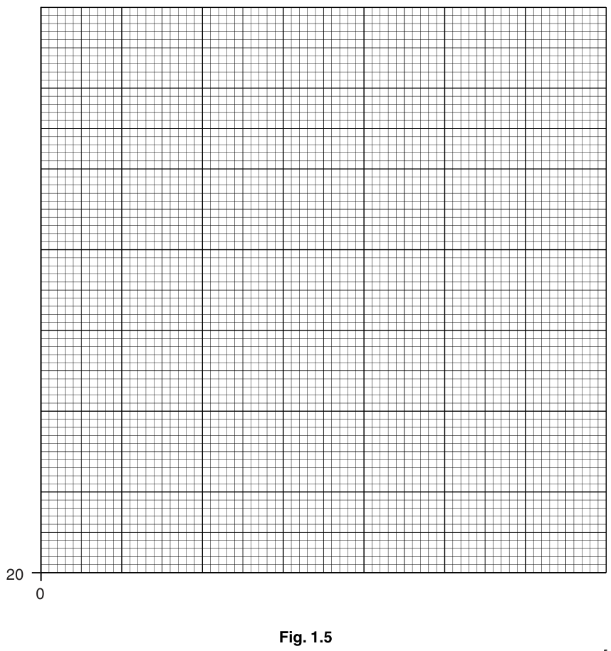
On Fig. 1.5, plot the graph of on the y-axis against on the x-axis.
Start your graph at and .
Draw a smooth curve of best fit.
Working
- Axes and labels:
- -axis: Speed , starting at . Scale: (so ).
- -axis: Depth , starting at . Scale: (so ).
- Points to plot:
- Line: A single smooth best-fit curve drawn through the plotted points, starting from and extending smoothly through with a decreasing gradient.
Answer
Graph plotted with correctly labelled axes, appropriate linear scales occupying more than half the grid, accurate points within small square, and a smooth curve of best fit.
Graph of v against d plotted with smooth curve of best fit
Walkthrough
To achieve full marks on the graph (4 marks total):
- Axes (B1): Label the horizontal -axis as and the vertical -axis as .
- Scales (B1): The question specifies starting at and .
- For the -axis, with going up to , a convenient linear scale is (1 large grid square) .
- For the -axis, with ranging from to , a scale of (1 large grid square) spans from to across 7 large squares, occupying well over half the vertical grid.
- Plotting points (B1): Each point from the table must be plotted with a small neat cross '' or a dot in a small circle '' to within of a small square ():
- Line of best fit (B1): Draw a single, continuous, smooth curve that shows a decreasing gradient as increases. The curve must not be forced into a straight line or drawn with 'point-to-point' jagged segments.
Key Takeaways
- Always check specified starting values for the axes (here: ).
- Choose scales that make plotting and reading easy (multiples of 1, 2, or 5).
- Best-fit curves should be drawn in a single smooth motion without kinks, doubling, or feathering.
Common Mistakes
- Forcing a straight line of best fit when the trend is clearly curved.
- Starting the -axis at instead of the specified , resulting in a compressed scale.
- Plotting large, blurry blobs instead of precise small crosses.
Things to Be Careful About
- Double-check scale intervals: each small square () on the -axis represents , and on the -axis represents .
Suggest a possible reason why the student cannot take readings for greater than .
Answer
The tray is not deep enough, so adding more water would cause it to spill over the sides when lifted or when the wave travels.
The tray is not deep enough / water would spill out over the edges
Walkthrough
When lifting and lowering the tray to create a wave, water sloshes near the edges. If the depth exceeds , the water level approaches the rim of the tray, causing water to spill out when the tray is tilted or when the wave reflects at the end walls. Another valid reason is that at larger depths the wave travels too fast, making the travel time too small to measure reliably.
Key Takeaways
- Experimental range is often constrained by physical boundaries of the equipment (dimensions, capacity, overflowing, limits of sensor/human reaction).
Common Mistakes
- Stating that the ruler is not long enough (the ruler is , which is far greater than ). Focus on the tray or water dynamics.
Things to Be Careful About
- Ensure the suggested limitation is physically realistic based on the apparatus shown in Fig. 1.1.
Using your graph, suggest how the speed varies with depth for very large values of .
Answer
The gradient of the curve decreases as increases, suggesting that for very large depths, the speed becomes constant (or the increase in speed becomes negligible).
The speed becomes constant / the increase in speed becomes smaller / gradient decreases
Walkthrough
Observing the plotted curve on the graph:
- Between and , the speed increases by .
- Between and , the speed increases by only .
The slope (gradient ) is continuously decreasing as depth increases. Extrapolating this trend to very large depths indicates that the rate of increase of speed tends to zero, meaning the speed will level off and approach a constant value (independent of depth in deep water).
Key Takeaways
- A curve flattening out (decreasing slope) indicates that the dependent variable is approaching a plateau or constant value as the independent variable increases.
Common Mistakes
- Claiming the speed will decrease to zero.
- Claiming the speed increases proportionally or infinitely without noticing the flattening curvature.
Things to Be Careful About
- Reference the shape of the graph (gradient decreasing / curve leveling off) to justify the conclusion.
The rest of this paper
3 more questions- Q2Analysis, Conclusions and Evaluation · Experimental Contexts · Use of Techniques, Apparatus and Materials6M
- Q3Observations and Measurements · Analysis, Conclusions and Evaluation5M
- Q4Experimental Contexts · Use of Techniques, Apparatus and Materials · Observations and Measurements7M