The Normal Distribution Revision Notes — 9709 Paper 5

topic	marks/paper
Discrete Random Variables	13.2
The Normal Distribution	11.6
Probability	11.2
Permutations and Combinations	9.8
Representation of Data	9.3

sub-topic	parts	marks	sections
Solving problems using standardisation ( $Z$ -scores)	87	315	02–08
Normal approximation to the binomial, with continuity correction	30	142	09
The normal distribution as a model for a continuous variable	25	89	01

The normal distribution as a model for continuous data

Syllabus requirement · §5.5

“

understand the use of a normal distribution to model a continuous random variable, and use normal distribution tables

”

Discrete and continuous variables

A discrete random variable takes separate values you can list: the number of heads in 10 tosses can be $0, 1, 2, \dots, 10$ and nothing in between. Each value has its own probability, and the probabilities add up to $1$ (the Discrete Random Variables topic, 5.4).

A continuous random variable can take any value in a range. The mass of a bag of rice could be $1.48$ kg, $1.483$ kg, $1.4831$ kg, … There are infinitely many possible values packed into any interval, so the probability of hitting one exact value is $0$ :

\mathrm{P}(X = 1.48) = 0 \quad \text{for a continuous } X

Probabilities only make sense for intervals, such as $\mathrm{P}(1.4 < X < 1.5)$ . A continuous distribution is described by a curve, and

\mathrm{P}(a < X < b) = \text{the area under the curve between } a \text{ and } b

The total area under the curve is $1$ , because $X$ is certain to take some value.

One useful consequence: since a single value has probability $0$ , including or excluding an endpoint makes no difference. $\mathrm{P}(X < 5)$ and $\mathrm{P}(X \leqslant 5)$ are the same number for a continuous variable. (This is not true for a discrete variable, and §09 is all about that difference.)

The normal curve

Many measured quantities (heights, masses, lengths, times) cluster around a central value, with values further from the centre becoming steadily rarer, equally on both sides. The normal distribution is the model for this. Its curve is the symmetric bell shape below. We write

X \sim \mathrm{N}(\mu, \sigma^2)

read " $X$ is normally distributed with mean $\mu$ and variance $\sigma^2$ ". Here:

$\mu$ (the Greek letter "mu") is the mean, the centre of the bell;
$\sigma$ (the Greek letter "sigma") is the standard deviation, which measures how spread out the values are;
$\sigma^2$ is the variance. The second number inside $\mathrm{N}(\ ,\ )$ is always the variance, not the standard deviation.

Properties you can read off the picture:

the curve is symmetric about $\mu$ , so exactly half the area is on each side: $\mathrm{P}(X < \mu) = \mathrm{P}(X > \mu) = 0.5$ ;
the mean, median and mode are all equal to $\mu$ ;
the curve never quite touches the axis, but almost all of the area lies within $3\sigma$ of the mean (between $\mu - 3\sigma$ and $\mu + 3\sigma$ ).

The normal curve: symmetric about μ, with mean = median = mode, total area 1, and almost all of the area within 3σ of the mean.

Changing $\mu$ slides the whole curve left or right without changing its shape. Changing $\sigma$ changes the spread: a larger $\sigma$ gives a wider, flatter curve, and a smaller $\sigma$ a narrower, taller one. The curve has to get taller as it gets narrower because the total area must stay equal to $1$ .

Left: same σ, different μ (the curve slides). Right: same μ, different σ (the curve stretches; the narrow one is taller because each area is 1).

Reading the notation

For each random variable, state the mean and the standard deviation.

(a) $X \sim \mathrm{N}(20, 9)$ (b) $Y \sim \mathrm{N}(5.2, 1.5^2)$ (c) $W \sim \mathrm{N}(31.4, 3.6)$

(d) For the variable in (a), write down $\mathrm{P}(X = 20)$ and $\mathrm{P}(X \leqslant 20)$ .

Show full working

1
(a) Read the two numbers. In $\mathrm{N}(20, 9)$ the first number is the mean and the second is the variance: $\mu = 20, \qquad \sigma^2 = 9$
Always say out loud which number is which: mean first, variance second.
2
Square-root the variance to get the standard deviation. $\sigma = \sqrt{9} = 3$
Every later calculation divides by σ, so this is the number you will actually use. Dividing by 9 instead of 3 is a common way to lose a whole question.
3
(b) The variance is written as a square. $\mathrm{N}(5.2, 1.5^2)$ has variance $1.5^2$ , so $\mu = 5.2, \qquad \sigma = 1.5$
Writing the variance as 1.5² is Cambridge's way of handing you σ directly. Don't square 1.5 and then forget to undo it.
4
(c) A variance that is not a perfect square. $\mathrm{N}(31.4, 3.6)$ has $\sigma^2 = 3.6$ , so $\mu = 31.4, \qquad \sigma = \sqrt{3.6} = 1.897\ldots$
Keep σ = √3.6 on the calculator rather than typing a rounded 1.9, so later answers stay accurate.
5
(d) A single exact value. $X$ is continuous, so $\mathrm{P}(X = 20) = 0$
There is no area above a single point on the axis.
6
Including the endpoint changes nothing. $\mathrm{P}(X \leqslant 20) = \mathrm{P}(X < 20)$
The single value 20 has probability 0, so adding it to the region adds no area.
7
Use symmetry about the mean. $20$ is the mean, so the area to its left is half the total: $\mathrm{P}(X \leqslant 20) = 0.5$
Exactly half of the area lies on each side of the mean.

Answer

(a) $\mu = 20$ , $\sigma = 3$ . (b) $\mu = 5.2$ , $\sigma = 1.5$ . (c) $\mu = 31.4$ , $\sigma = \sqrt{3.6} \approx 1.90$ . (d) $\mathrm{P}(X = 20) = 0$ and $\mathrm{P}(X \leqslant 20) = 0.5$ .

Sketching normal curves

A sketch question gives you one or more distributions and asks for their curves on one diagram. The mark scheme looks for three things, so build each curve from them:

the peak sits directly above the mean $\mu$ ;
the curve runs down to the axis about $3\sigma$ either side, so it spans roughly $\mu - 3\sigma$ to $\mu + 3\sigma$ ;
relative heights: a curve with a smaller $\sigma$ is narrower and taller; two curves with the same $\sigma$ have the same shape and height.

Sketching two curves on one diagram

$A \sim \mathrm{N}(10, 4)$ and $B \sim \mathrm{N}(16, 1)$ . Describe how you would sketch both curves on one diagram with the horizontal axis from $0$ to $20$ .

Show full working

1
Find each standard deviation. $A$ has variance $4$ , so $\sigma_A = \sqrt{4} = 2$ . $B$ has variance $1$ , so $\sigma_B = 1$ .
The spread of a sketch depends on σ, not on the variance.
2
Where does curve $A$ start and finish? $\mu_A - 3\sigma_A = 10 - 6 = 4, \qquad \mu_A + 3\sigma_A = 10 + 6 = 16$ So $A$ is a bell centred at $10$ , meeting the axis at about $4$ and $16$ .
Three standard deviations either side covers almost all of the area, so this is where the curve should visibly reach the axis.
3
Where does curve $B$ start and finish? $\mu_B - 3\sigma_B = 16 - 3 = 13, \qquad \mu_B + 3\sigma_B = 16 + 3 = 19$ So $B$ is centred at $16$ and runs from about $13$ to $19$ .
Same rule, different numbers.
4
Compare the heights. $B$ has half the standard deviation of $A$ , so $B$ is half as wide and must be about twice as tall to enclose the same area of $1$ .
This is the mark examiners most often withhold: a narrower curve drawn at the same height as a wider one.

Answer

$A$ : a bell with its peak above $10$ , reaching the axis near $4$ and $16$ . $B$ : a narrower bell, about twice as tall, with its peak above $16$ , reaching the axis near $13$ and $19$ .

A sketch question from a real paper

9709/61 O/N 2013 Q13 marks

It is given that $X \sim \mathrm{N}(30, 49)$ , $Y \sim \mathrm{N}(30, 16)$ and $Z \sim \mathrm{N}(50, 16)$ . On a single diagram, with the horizontal axis going from 0 to 70, sketch three curves to represent the distributions of $X$ , $Y$ and $Z$ .

Show full working

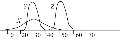
The mark scheme's own sketch: X and Y share a centre at 30, Y is narrower and taller, and Z is the same shape as Y moved to 50.

1
Standard deviations. $\sigma_X = \sqrt{49} = 7, \qquad \sigma_Y = \sqrt{16} = 4, \qquad \sigma_Z = \sqrt{16} = 4$
The second number in each bracket is a variance, so take square roots first.
2
Curve $X$ . Peak above $30$ . It spans about $30 - 3(7) = 9$ to $30 + 3(7) = 51$ .
The mark scheme accepts X running roughly from 10 to 50 (or 15 to 45).
3
Curve $Y$ . Same centre, $30$ , but $\sigma_Y = 4$ is smaller than $\sigma_X = 7$ , so $Y$ spans only about $18$ to $42$ and is taller than $X$ .
One mark is for 'same mean as X but higher and thinner'. Both words matter.
4
Curve $Z$ . Same variance as $Y$ , so it is an identical shape (same width, same height), with its peak moved to $50$ . It spans about $38$ to $62$ .
Z and Y differ only in μ, and changing μ only slides a curve.

Answer

Three bells: $X$ centred at $30$ , wide and low; $Y$ centred at $30$ , narrower and taller than $X$ ; $Z$ exactly the shape of $Y$ but centred at $50$ .

In a sketch, label each curve and its mean on the axis. Relative width and height are what earn the marks, not exact heights.

When is a normal model suitable?

A normal distribution is a sensible model for data that is:

continuous (measurements such as mass or time, not counts);
symmetric, with a single peak in the middle;
tailing off evenly on both sides, with few values far from the centre.

It is not suitable for data that is clearly skewed (for example waiting times with a long right tail), has two peaks, or is a small whole-number count. If a question shows you a diagram of the data and asks whether a normal model fits, give two features: "symmetric" plus one more ("peaks in the middle" or "tails off on both sides").

Judging a model from a frequency table

The masses, $m$ grams, of 100 tomatoes are summarised below. Is a normal distribution a suitable model? Give reasons.

$m$	60–70	70–80	80–90	90–100	100–110	110–120
frequency	3	16	31	30	17	3

Show full working

1
Is the variable continuous? Mass is a measurement, so yes.
A count such as 'number of seeds' would already rule out a normal model.
2
Where is the peak? The biggest frequencies, $31$ and $30$ , are in the two middle classes, so there is a single peak in the middle.
A normal curve has one peak, at the mean.
3
Is it symmetric? Reading outwards from the middle: $31$ and $30$ , then $16$ and $17$ , then $3$ and $3$ . The two sides almost match.
Pair up classes the same distance from the centre and compare them.
4
Do the tails thin out? Yes: only $3$ tomatoes in each end class.
Few values far from the centre, on both sides.
5
Conclude, with two reasons. A normal model is suitable: the masses are symmetrical about the middle and peak in the centre, tailing off at both ends.
Symmetry plus one more feature is what earns both marks.

Answer

Yes: the data is continuous, roughly symmetrical, with a single central peak and thin tails on both sides.

Naming a model from a stem-and-leaf diagram

9709/62 F/M 2017 Q4(ii)2 marks

The weights in kilograms of packets of cereal were noted correct to 4 significant figures. The following stem-and-leaf diagram shows the data.

Key: $748 \mid 5$ represents $0.7485\text{ kg}$ .

Name a distribution that might be a suitable model for the weights of this type of cereal packet. Justify your answer.

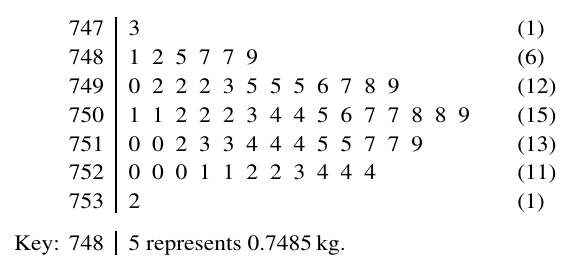
The printed stem-and-leaf diagram: 59 weights, with the row frequencies in brackets.

Show full working

1
Look at the shape. Reading the row frequencies down the page: $1, 6, 12, 15, 13, 11, 1$ . They rise to a single peak in the middle (the $750$ row) and fall away on both sides.
A stem-and-leaf diagram turned on its side is a bar chart, so the shape of the distribution can be read directly.
2
Check symmetry and tails. The two extremes are both $1$ , and the frequencies fall away on both sides of the peak, so the shape is roughly symmetrical.
Symmetry plus a peak in the middle is exactly the picture of a normal curve.
3
Name the model and give two reasons. A normal distribution: the data is (roughly) symmetrical and peaks in the middle, tailing off at both ends.
The mark scheme requires 'symmetrical' plus another reason for the second mark.

Answer

A normal distribution, because the weights are roughly symmetrical and peak in the middle (tailing off quickly at both ends).

Common mistakes

Reading $\mathrm{N}(20, 9)$ as "mean 20, standard deviation 9"
The second number is the variance: $\sigma = \sqrt{9} = 3$
Every mark scheme in this topic says 'not σ², not √σ' next to the standardising mark.
Drawing a narrow and a wide normal curve at the same height
The narrower curve (smaller $\sigma$ ) must be taller, since both areas are $1$
Sketch questions award a separate mark for 'higher and thinner'.
Justifying a normal model with "symmetrical" alone
Give two features: symmetrical and peaks in the middle (or tails off at both ends)
The mark scheme needs symmetry plus another reason.

Your turn

1
State the mean and standard deviation of (a) $\mathrm{N}(12, 0.25)$ , (b) $\mathrm{N}(-3, 2^2)$ , (c) $\mathrm{N}(100, 50)$ .
Stuck? Show hint
Mean first, variance second. Square-root the variance.
Show solution
1. 1
  (a) $\mu = 12$ and $\sigma^2 = 0.25$ , so $\sigma = \sqrt{0.25} = 0.5$
  The square root of a number less than 1 is bigger than the number.
2. 2
  (b) $\mu = -3$ and the variance is written as $2^2$ , so $\sigma = 2$
  A negative mean is fine. Only σ has to be positive.
3. 3
  (c) $\mu = 100$ and $\sigma^2 = 50$ , so $\sigma = \sqrt{50} = 7.07 \ (\text{3 s.f.})$
  Not a perfect square, so keep the exact value on your calculator.
Answer
(a) $12$ and $0.5$ ; (b) $-3$ and $2$ ; (c) $100$ and $\sqrt{50} \approx 7.07$ .
2
For each variable, say whether a normal distribution is likely to be a suitable model, with a reason. (a) The heights of adult women in a large city. (b) The number of heads when a coin is tossed 3 times. (c) The time customers wait in a queue, where most wait under 2 minutes but a few wait over 20 minutes.
Stuck? Show hint
Is it continuous? Is it symmetric with one central peak?
Show solution
1. 1
  (a) Suitable: height is continuous, and heights cluster symmetrically around an average with few very short or very tall people.
  This is the textbook normal situation.
2. 2
  (b) Not suitable: the number of heads is a discrete count with only four possible values ( $0$ , $1$ , $2$ , $3$ ). It is binomial, $\mathrm{B}(3, 0.5)$ .
  A normal model needs a continuous variable (or, as in §09, a binomial with a large n).
3. 3
  (c) Not suitable: the waiting times are heavily skewed, bunched near $0$ with a long tail to the right, so they are not symmetric.
  A normal curve has equal tails on both sides.
Answer
(a) Yes: continuous and symmetric about a central value. (b) No: a small discrete count. (c) No: strongly skewed.

Practise the normal distribution as a modelReal past-paper questions · Normal distribution as a model for continuous random variables

Checking your access…

Can you do all of these?

Sketch the curve and shade the region before any algebra; decide whether the answer is above or below 0.5
N(μ, σ²): the second number is the variance; divide by σ, never by σ² or √σ
Write the standardising line with the numbers substituted: the first method mark is for it
Φ is the area to the left: a right tail is 1 − Φ, and Φ(−z) = 1 − Φ(z)
Use the ADD columns for a third decimal place of z, and quote table values to 4 d.p.
For 0.75, 0.9, 0.95, 0.975, 0.99 use the critical values 0.674, 1.282, 1.645, 1.960, 2.326 exactly
Expected number = n × p with p to at least 4 s.f.; give a single whole number, no '≈'
'Within k of the mean' is 2Φ(k) − 1; 'more than k from the mean' is both tails; 'above' is one tail
A distance given in standard deviations is already the z-value
Working backwards, the sign of z comes from where the boundary is: above μ positive, below μ negative
Equate the standardised expression to a z-value, never to a probability
Signs must be consistent: x₁ − μ and z have the same sign, and σ must come out positive
For an interval with one unknown end, add the known tail to the slice to get the area to the left
Two unknowns: two z-values, each with its own sign; clear fractions, subtract to remove μ, solve for σ, substitute back
A given relationship between μ and σ is the second equation: substitute it at once; with a boundary of 0 it cancels
Binomial approximation: evaluate np and nq and compare both with 5
Mean np, variance npq, standard deviation √(npq)
Continuity correction: list the whole numbers wanted and cut half-way to the first one not wanted

Now do the questions

112 real Paper 5 parts from 2021–2025, sorted by difficulty, with mark schemes

Discrete Random Variables

The Normal Distribution

The normal distribution as a model for continuous data

Discrete and continuous variables

The normal curve

Sketching normal curves

When is a normal model suitable?

The standard normal distribution and the Φ table

Standardising to find a probability

Can you do all of these?

The normal distribution as a model for continuous data

Discrete and continuous variables

The normal curve

Sketching normal curves

When is a normal model suitable?

The rest of this note

Can you do all of these?