Probability density functions: properties and finding constants
“
understand the concept of a continuous random variable, and recall and use properties of a probability density function. Notes: for density functions defined over a single interval only; the domain may be infinite.
A probability density function (pdf), , describes a continuous random variable — one that can take any value in an interval, not just whole numbers. is not itself a probability (it can even exceed ); it's a density, and probability comes from the area underneath it. Two properties define any valid pdf, over its support (the interval of -values where can actually fall — everywhere else):
The first is just common sense — a density can't be negative. The second is the continuous version of "a distribution table's probabilities sum to ": the whole area under the curve, across every value could take, must account for all the probability there is.
Almost every question gives you a support with two ordinary numbers at its ends, like . The syllabus does allow it to be unbounded — its own example is for , and , so that really is a pdf. Nothing about the method changes: the upper limit is just , and a term like goes to as .
Probability is the shaded area under f(x) — and a single point, having zero width, has zero area and therefore zero probability.
P(X = c) = 0 for any continuous X
Because a single value has zero width, it contributes zero area, so for every . This has a genuinely useful consequence: for a continuous variable, , , and are all equal — unlike the discrete case (§5.4/§6.1), strict and non-strict inequalities never need separate treatment here.
Finding an unknown constant from total area = 1
A random variable has probability density function Find the value of the constant .
Show full working
- 1
Step 1 — write the total-area condition for this support. Since outside , the whole area is the integral from to :
- 2
Step 2 — integrate, treating as a constant multiplier.
- 3
Step 3 — substitute the limits.
- 4
Step 4 — solve for .
.
Write the total-area equation with the correct support limits before integrating anything — an unknown constant is found from exactly one equation, so getting the limits right the first time avoids redoing the whole integral.
The same idea with a second unknown left in the answer
The random variable has probability density function where and are positive constants. Show that .
Show full working
- 1
Step 1 — write the total-area condition.
- 2
Step 2 — take the constant outside the integral, then integrate .
- 3
Step 3 — substitute the limits.
- 4
Step 4 — simplify the power of (), then solve for .
, as required.
When the answer is a 'show that', every intermediate line — the integrated expression, the substituted limits, the simplification — must actually appear; quoting only the final equality earns no method credit.
Verifying a pdf from a graph — no calculus needed
The graph of the function is a straight line segment from to . Show that could be a probability density function.
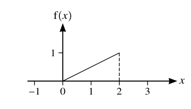
The figure printed with the question: f is the line segment from (0, 0) to (2, 1), and zero everywhere else.
Show full working
- 1
Step 1 — recall what has to be shown. "Could be a pdf" means exactly two things, and the mark scheme awards one mark for each: everywhere, and the total area under the graph is . So the answer needs both, not just the more interesting one.
Candidates routinely compute the area, get 1, and stop — throwing away the second mark. The non-negativity line is one sentence and is worth the same as the whole area calculation.
- 2
Step 2 — check non-negativity. The segment runs from up to , so it lies on or above the -axis for every in , and outside. Hence for all — the first condition holds.
- 3
Step 3 — identify the shape under the graph. From to with the -axis beneath it, the region is a right-angled triangle: base along the -axis of length , and vertical height at .
- 4
Step 4 — find the total area with the triangle formula.
The mark scheme explicitly allows either ½ × 2 × 1 or ∫₀² ½x dx — so the geometry route earns full marks and takes one line instead of four. Recognising the shape first can save the whole calculation.
- 5
Step 5 — state the conclusion. The total area is exactly and throughout, so both defining conditions are satisfied and could be a probability density function.
everywhere, and the area under the graph is — so satisfies both conditions and could be a pdf.
Before reaching for an integral, check whether the region under the graph is a standard shape — a triangle, a rectangle, a semicircle — whose area formula is faster and less error-prone than setting up ∫f(x)dx from scratch. And on any 'show it could be a pdf' part, always write both conditions down.
The same two conditions, used in reverse to find an unknown
The graph of the function is a semicircle, centre , entirely above the -axis. Given that is a probability density function, find the radius of the semicircle.
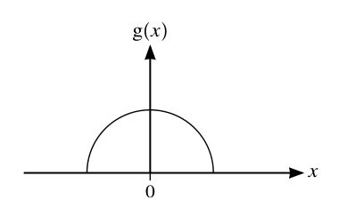
The figure printed with the question: g is the upper half of a circle centred at the origin — so its radius is also the half-width of the support.
Show full working
- 1
Step 1 — see which way round the question runs. The previous part checked that the area was . Here we are told is a pdf, so the area is — and that single fact is what pins down the one unknown, the radius.
This is the standard move of the whole section: 'total area = 1' is one equation, so it determines exactly one unknown. Whether that unknown is a constant k or a radius r makes no difference to the method.
- 2
Step 2 — write the area of the region in terms of the unknown. Call the radius . The graph is the upper half of a circle of radius , so the region between it and the -axis is a semicircle, of area .
- 3
Step 3 — set that area equal to .
- 4
Step 4 — multiply both sides by , then divide by .
- 5
Step 5 — take the square root, keeping the positive root, since a radius cannot be negative.
(3 s.f.).
A circular or semicircular density looks alarming but never needs integration — it is there precisely so that the area formula does the work. Note also that the semicircle's radius doubles as the support: this X runs from −r to r.
Using symmetry, without any integration at all
If a pdf's graph is symmetric about some vertical line , then any two intervals that reflect onto each other across automatically have equal probability. Two facts follow, and between them they answer a surprising number of questions with no integration at all:
- Mirror-image intervals have equal probability. Measure each interval's distance from the line ; if they match, so do the probabilities.
- Each side of the line carries exactly half the area. So everything below has probability , and so does everything above it.
A quick invented case to see both at work. Suppose is symmetric about and you are told .
- The interval from to reaches units above the centre. Its mirror image reaches units below, i.e. from to — so as well, by fact 1.
- The whole left half, below , has probability by fact 2. The piece of it from to accounts for , so what remains — the tail below — must be
- And then .
No integral, and indeed no formula for was ever needed. The worked example below is the same two moves on a real paper.
A probability found purely from symmetry
The graph of the probability density function of a random variable is symmetrical about the line . It is given that . Using only this information, show that .
Show full working
- 1
Step 1 — use symmetry about to find the reflection of the given interval. The interval to is units to the right of the line of symmetry; reflecting it across gives the interval to , units to the left. By symmetry, these have equal probability:
- 2
Step 2 — use the fact that the two halves of the total area, split at the line of symmetry , are each exactly . So the "far tail" beyond (i.e. ) has probability
Since x = 2 is the centre of symmetry, exactly half the total area of 1 lies on each side of it — the interval from −1 to 2 accounts for part of the left half, and whatever's left over is the tail beyond −1.
- 3
Step 3 — assemble as the complement of that far tail.
, as required.
Reflecting an interval across a stated line of symmetry, then using 'each half of the curve has area ½', very often answers a probability question with no integral at all — look for this before setting one up.
Sketching the density of a linear transformation
§6.2 gave the mean and variance of in terms of 's. The graph of 's density follows the same idea, and Cambridge asks for it directly as a sketch. Every value that could take becomes the value for , so take 's density graph and, in this order (for a positive constant ):
- stretch it horizontally by a factor of — the happens to first, so the support's width multiplies by ;
- then shift it horizontally by — the is applied to the already-stretched picture, sliding it right if and left if ;
- and divide its height by — this is the part that's easy to forget, and it's forced by the total area staying equal to : the stretch multiplied the width by , so the height must be divided by to leave width height unchanged.
The order in steps 1 and 2 matters. Stretching first and then shifting sends to , which is what actually is. Shifting first and then stretching would send to — a different graph, in the wrong place.
Y = 2X − 1: the support doubles in width (4 → 8) and the height halves (0.25 → 0.125) — area stays exactly 1 either way.
Sketching g(y) for Y = aX + b from a known f(x)
A random variable has the constant density for (and elsewhere). The random variable . State the probability density function of , and describe how its graph compares with 's.
Show full working
- 1
Step 1 — find the new support, mapping each endpoint of 's support through . So takes values on .
Every x-value maps through the same rule that defines Y — the endpoints of the support are not a special case, they transform exactly like every other point.
- 2
Step 2 — find the new width, and compare with the old. Old width ; new width — exactly double, matching the multiplier .
- 3
Step 3 — find the new height, using the fact that width height must still equal .
This is exactly the old height (0.25) divided by a = 2 — doubling the width and halving the height are the same statement, both forced by total area = 1.
- 4
Step 4 — write the density of explicitly.
- 5
Step 5 — describe the graph. Compared with , 's graph is the same flat shape, shifted and stretched: twice as wide, positioned from to instead of to , and exactly half as tall.
for — twice as wide and half as tall as .
This 'sketch the transformed density' question is common with X's own graph given only as a picture (often a symmetric quadratic or triangle) rather than a formula — the same three moves apply regardless of the shape: map the endpoints through y = ax + b, stretch the width by a, and divide the height by a to keep the area at 1.
When you're given the mean and variance instead of the rule
The exam more often gives you the effect of the transformation — a new mean and a new variance — and leaves you to deduce the picture. Two facts do all the work, and they are worth learning as a pair:
- The mean says where the graph sits. Changing slides the whole graph sideways without altering its shape.
- The variance says how wide it is. Variance is measured in squared units, so it is the standard deviation — the square root — that scales with width. Multiply the variance by and the width halves, because .
Then, as always, the height moves opposite to the width so that the area stays : halve the width and the height doubles.
Sketching a transformed density from its new mean and variance
The diagram shows the graph of the probability density function of a random variable that takes values between and only. The graph is symmetrical about the line , and between and it is a quadratic curve with maximum height at .
(a) The random variable is such that and . Sketch a quadratic graph for the probability density function of .
(b) The random variable is such that and . Sketch a quadratic graph for the probability density function of .
![The given density of X: a quadratic on [−1, 3], symmetric about x = 1, peaking at 0.375. The exam supplies blank grids of the same size to sketch on.](https://pub-2f44901a36d54bf99ce3730cc4edf6c7.r2.dev/9709/2022-Oct-Nov/9709_w22_qp_61_1.png)
The given density of X: a quadratic on [−1, 3], symmetric about x = 1, peaking at 0.375. The exam supplies blank grids of the same size to sketch on.
Show full working
- 1
Step 1 — read off what you need about itself. The graph is symmetric about , so . Its support is , so its width is , and its greatest height is . Those three numbers — centre , width , height — are all that either sketch depends on.
You are never asked for Var(X) as a number, and you could not easily find it from the picture anyway. Only the CHANGE in variance matters, so work in ratios throughout.
- 2
Step 2 — (a) find 's centre. , so 's graph is centred on instead of — shifted one unit to the right.
- 3
Step 3 — (a) find 's width. — the variance is unchanged, so the spread is unchanged and the width is still . A width of centred on runs from to .
Equal variance means this is a pure slide, with no stretching at all. Students often assume that because the mean doubled the graph must also stretch — but the mean and the variance are independent instructions, and only the variance controls width.
- 4
Step 4 — (a) find 's height. The width did not change, so the height must not change either, or the area would stop being . The peak stays at height , now sitting above .
- 5
Step 5 — (a) describe the sketch. The same quadratic shape, from to , touching the axis at both ends, with its maximum at the point .
- 6
Step 6 — (b) find 's centre. , so this graph does not move — it stays centred on .
- 7
Step 7 — (b) find 's width. . Width follows the standard deviation, not the variance, so take the square root: The width is halved, from to . A width of centred on runs from to .
This square root is the single most common error in the question. Scaling the width by ¼ instead of ½ would give the support [0.5, 1.5] — a graph the mark scheme rejects outright.
- 8
Step 8 — (b) find 's height. The width halved, so the height must double to keep the area at :
- 9
Step 9 — (b) describe the sketch. The same quadratic shape but narrower and taller, from to , with its maximum at the point .
(a) A quadratic curve from to , maximum at . (b) A quadratic curve from to , maximum at .
Reduce every sketch of this type to three numbers — centre, width, height — and get them in that order. Centre comes from the mean; width from the SQUARE ROOT of the variance ratio; height from 'area must stay 1'. The mark scheme here awards the endpoints and the coordinates of the maximum, so label those explicitly on your sketch and don't worry about drawing a beautiful curve.
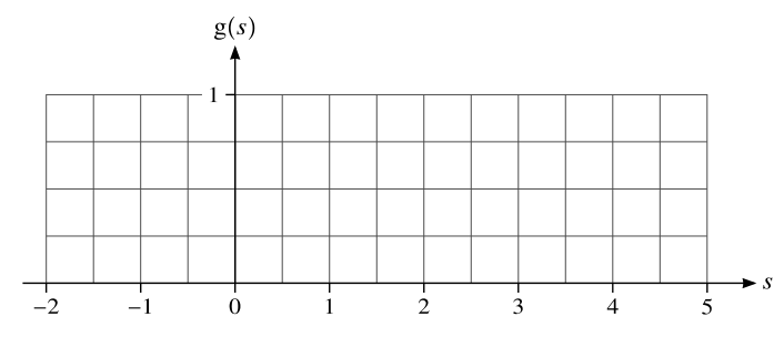
The grid the exam gives you for part (a). It is printed at the same scale as the original — from to — so your curve must start on the axis at , return to it at , and peak at , a shade over a third of the way up to the marked .
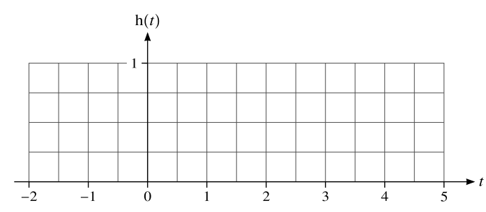
The identical grid for part (b). Here the curve is squeezed into and stretched upwards to a peak of — visibly narrower and twice as tall as the one above, which is exactly the point the examiner is checking.
Integrating over limits that don't match the pdf's actual support
Always integrate over exactly the interval where is non-zero, as stated in the question
The density is 0 outside its support by definition — integrating too far (or not far enough) silently adds or omits area that was never really there.
Treating , the height of the density at a point, as if it were
always, for any continuous — is a density, not a probability
f(x) can even be greater than 1 at some points; it only becomes a probability once it's integrated over a range with actual width.
When sketching 's density, scaling the height by instead of
Width multiplies by ; height divides by — they move in opposite directions, so the area stays
Scaling both width and height by a would multiply the total area by a², so the total probability would come out as a² instead of 1 — right only in the trivial case a = 1. Whenever you sketch a transformed density, check the area of your sketch is still 1 before moving on.
- 1
Check across the stated support (or find the support from where a given expression is ).
- 2
Check for a standard area shape first — a rectangle, triangle or semicircle's formula beats setting up an integral.
- 3
Otherwise, integrate over the support and set the result equal to .
- 4
Solve for the unknown constant.
- 5
Check for symmetry before doing any further work — it can hand you (§03) or a probability (this section) for free.
Your turn
- 1
A random variable has probability density function for , and otherwise. Find the value of .
Stuck? Show hint
Write the total-area condition ∫₀⁶ kx dx = 1, integrate, then solve for k.
Show solution
- 1
Step 1 — write the total-area condition over the support .
- 2
Step 2 — take the constant outside and integrate .
- 3
Step 3 — substitute the limits.
- 4
Step 4 — solve for .
- 5
Step 5 — sanity-check with the triangle. The region under is a right-angled triangle of base and height , so its area is — the same , confirming Step 3.
Answer.
- 1
- 2
The probability density function of is symmetric about . Given , find .
Stuck? Show hint
Reflect the interval "X < 7" (i.e. more than 3 below the centre) across x = 10 to find its mirror-image interval.
Show solution
- 1
Step 1 — measure the given interval from the line of symmetry. The centre is , and is units to its left. So "" means " is more than units below the centre".
- 2
Step 2 — reflect that description across . Three units to the right of the centre is , so the mirror image of "" is "".
- 3
Step 3 — equate the two probabilities. Reflected intervals enclose mirror-image regions under a symmetric curve, so they have equal area:
Answer.
- 1
- 3
A random variable has the constant density for (and elsewhere). The random variable . State the probability density function of , including its support.
Stuck? Show hint
Map the endpoints x = 2 and x = 6 through w = 3x + 1 to find W's support, then use width × height = 1 to find the new height.
Show solution
- 1
Step 1 — map each endpoint of 's support through . So 's support is .
- 2
Step 2 — compare the widths. Old width ; new width . That is times as wide, matching the multiplier — a useful check that the endpoints were mapped correctly.
- 3
Step 3 — find the new height from width height . The density is still flat (stretching and sliding a horizontal line leaves it horizontal), so the graph is still a rectangle:
- 4
Step 4 — check against the rule. This is the old height divided by : ✓ — the width tripled, so the height was divided by three.
Answerfor .
- 1
The rest of this note
Can you do all of these?
P(X = c) = 0 for any continuous X — strict and non-strict inequalities never need separate treatment here
Integrate only over the interval where f(x) is actually non-zero — its stated support
Check for symmetry first — it can give E(X) and the median directly, with no integration at all
Only when the density is constant is probability interval width ÷ support width — any other shape needs the integral
Find E(X²) as its own separate integral, never by squaring E(X)
The median solves ∫f(x)dx = ½ from the lower support boundary — always check any algebraic root actually lies inside the support
The same equation with ½ replaced by any q locates any percentile — nothing else about the method changes, and the unknown can be the lower limit as easily as the upper
Write the rejection down. Whenever a quadratic or cubic gives two or more roots, say which you reject and why — that sentence is worth a mark on its own
Multiply the x in before choosing a method: x × 1/x² becomes 1/x (a logarithm), while x × cos πx cancels to nothing and needs integration by parts with u = x
P(X ⩽ m) = ½ by definition, with no work — so P(E(X) ⩽ X ⩽ m) is just ½ − P(X < E(X)), provided you check which of the two is larger
To verify a value lies between two numbers, evaluate at BOTH ends and say that the target is between the two results — one endpoint proves nothing
If a part says 'without calculation' or 'without integration', reuse the earlier answer — integrating afresh scores almost nothing; after a 'hence' it usually just caps the method marks
Symmetry gives mean = median for free; without it, expect them to differ — a long tail pulls the mean towards it more than the median